
Random Forests — wisdom of the crowd in Machine Learning
AI Literacy



There’s a particular kind of relief you feel when you stop trying to be “the genius” and instead try to be “the organizer of good judgments”.
You see it in everyday decisions. Picking a restaurant in a new neighborhood: one confident friend might push you into the loud, trendy place that photographs well but tastes like disappointment. A small group of friends - none of them perfect, some of them picky in different ways - often lands on something reliably good. Debugging a weird production issue: the one person who speaks first may sound persuasive, but a handful of engineers each tugging on a different thread (logs, metrics, recent deploys, networking, database behavior) is usually what gets you to the truth. Estimating a project timeline: the “optimist with certainty” is common; the “group that remembers different past failures” is useful.
Random forests are that pattern, turned into an algorithm.
A single decision tree can feel like a sharp mind: crisp rules, confident splits, clean explanations. And on training data, it often looks brilliant. But that brilliance is fragile - because a tree can accidentally turn a coincidence into a law. The random forest idea is to take many trees - each one trained under slightly different constraints - so that they disagree in productive ways. Then you combine them, and the disagreement cancels out a lot of the brittleness.
This post is about building a mental model you can actually use: not “random forest = many trees”, but “random forest = engineered diversity + aggregation”. If you understand that, the knobs, the trade-offs, and even the limitations become much easier to reason about without superstition.
🌳 If you've ever wondered why "just use a random forest" is such reliable advice on tabular data, this is the mental model - pass it to someone still fighting a single overfit tree.
A messy jury beats a single “genius”
Imagine you’re making a tough call: where to eat tonight, whether a bug is caused by caching or a race condition, how long a migration will take. One person speaks with confidence and tells a coherent story. It’s tempting to follow them - not because they’re correct, but because coherence is psychologically satisfying. A single narrative feels like understanding.
Now picture a small group instead. Each person has blind spots. One person always underestimates time. Another overweights aesthetics. Someone else is allergic to risk. But crucially, they’re not all wrong in the same direction. When you average their perspectives, you often get something calmer: fewer extreme decisions, fewer “we bet everything on one story” outcomes. The group’s strength isn’t that any member is perfect; it’s that their imperfections are varied.
That’s the core intuition behind random forests. A decision tree is a highly flexible model. It can carve the input space into lots of little regions and give each region its own prediction. If you let it, it will happily build a long chain of “if this, then that” rules that perfectly explain your training set. The problem is that the world doesn’t owe you the same quirks tomorrow.
A random forest takes many “pretty good” trees, encourages them to be different, and then combines their outputs. The combination step is important, but it’s not the whole story. The real magic is that the trees are pushed to become different kinds of wrong. Once you have that, averaging (for regression) or voting (for classification) turns the forest into a more reliable decision-maker than any single tree you could point to as “the best one”.
Why a single decision tree feels smart — and why it often isn’t
Decision trees are one of the most beginner-friendly models in machine learning, and that’s not an accident. They match the way humans naturally explain decisions: “If the user is new and their first session is short, show onboarding; otherwise, show the dashboard”. The logic is local, discrete, and narratable. You can draw it. You can walk a teammate through it. You can look at a split and argue about whether it “makes sense”.
They’re also expressive. A tree can model non-linear relationships without you manually inventing feature interactions. It can handle mixed feature types (continuous, categorical, binary) with minimal preprocessing. And if you keep splitting, it can fit complicated patterns very quickly.
The trap is that the same flexibility that makes trees expressive also makes them eager to over-explain the training data.
A tree is built by repeatedly choosing splits that improve some purity criterion (like reducing Gini impurity or entropy in classification, or reducing squared error in regression). Each split is a locally greedy choice. If you keep going deep, the tree keeps finding ways to isolate small pockets of the training set. Eventually, it can create leaves that contain only a handful of points - or even one point. At that depth, the tree is no longer learning a general rule; it’s learning a memory.
And memories feel like rules when you look at them as a flowchart.
This is why single trees are often high-variance models: small changes in the training data can produce a noticeably different tree. Change a few samples, and a key split might flip from “square footage” to “zipcode”, which then changes everything downstream. The tree didn’t become “worse” because it’s weak; it became fragile because it’s too responsive to the particularities of what it saw.
A forest keeps the appealing part - trees can capture complex patterns - while directly attacking that fragility.
The real problem isn’t weakness — it’s sameness
Ensembles are sometimes described as “many weak learners make a strong learner”. That’s not wrong, but it can hide the more important point: combining models only helps if they don’t all make the same mistakes.
If you have ten people estimating a project timeline, and they all use the same flawed assumption (“the API team will respond within a day”), averaging their estimates doesn’t fix the assumption. You just get a more confident wrong number. Volume is not wisdom. Diversity is.
In random forests, diversity matters because aggregation only reduces the parts of error that are not perfectly aligned across trees. If every tree latches onto the same misleading shortcut in the training data, voting and averaging just amplify that shortcut.
It’s worth making this intuition a little more concrete with a small piece of math - not as a proof to memorize, but as a way to see why correlation of errors is the real enemy.
A small variance calculation (with numbers you can redo)
Suppose each tree outputs a regression prediction. Write the prediction error of tree i as a random variable Xᵢ. Think of Xᵢ as “how far off tree i is” on a typical test point. If we average n trees, the averaged error is:
Now we ask: how variable is X̄? Start with:
Let S=Σᵢ Xᵢ. Then:
Assume each tree has the same error variance σ², and any pair has correlation ρ. Then:
There are n variance terms and n(n-1)/2 covariance pairs, so:
Divide by n²:
Now plug in numbers.
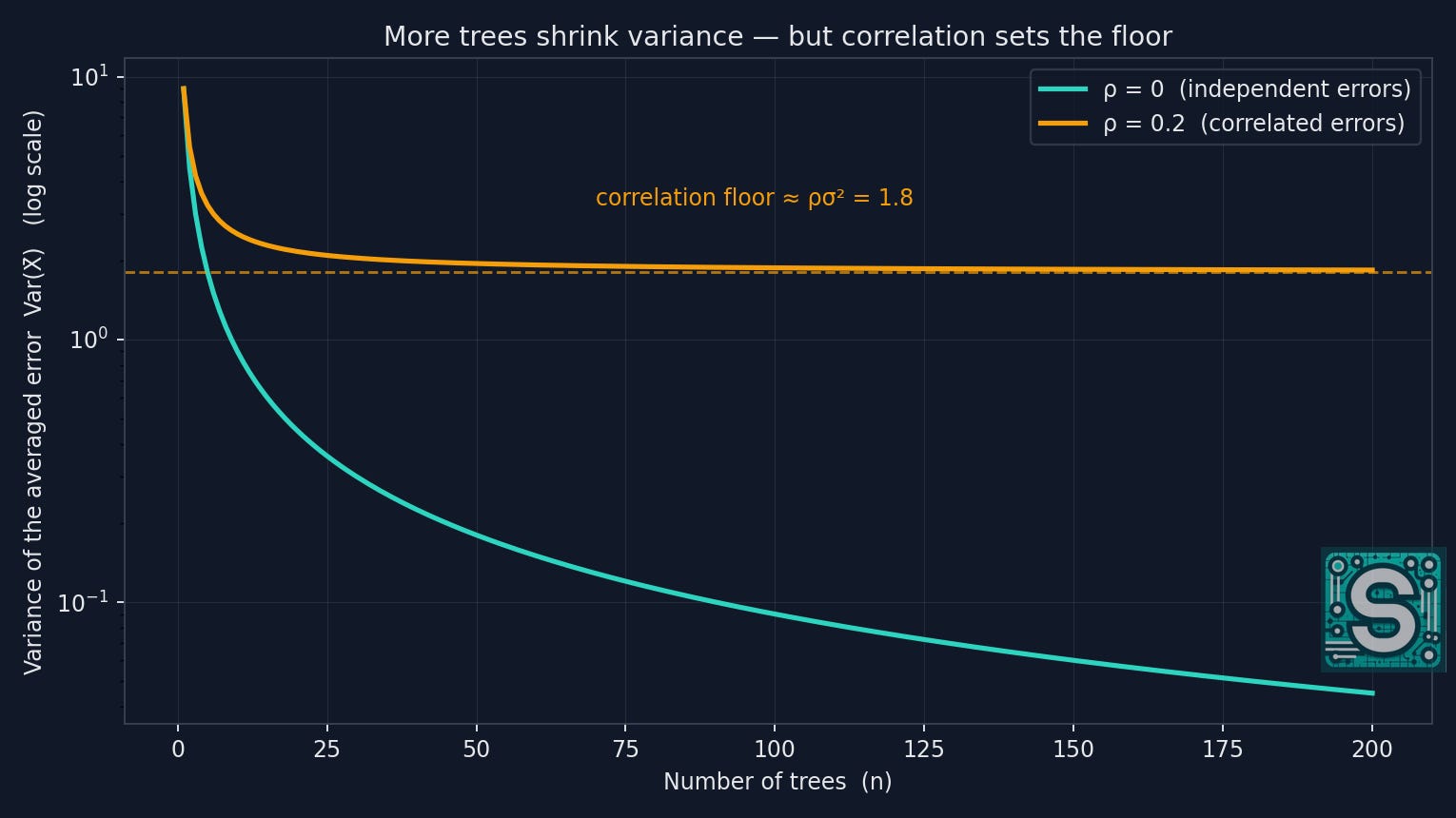
Example 1 (independent-ish trees). Given: σ²=9, n=100, ρ=0.
So the variance shrinks from 9 to 0.09. That’s a 100× reduction.
Example 2 (samey trees). Given: σ²=9, n=100, ρ=0.2.
Still better than 9, but nowhere near 0.09. The forest gained far less because the trees were too correlated - too similar in their errors.
That’s the heart of random forests: not “more trees”, but “less correlation between trees”.
How you get diversity without hand-holding the model
So how do we make trees disagree in useful ways, without manually designing different architectures or micromanaging each tree?
Random forests use two simple sources of randomness that are surprisingly effective.
First, each tree is trained on a slightly different dataset. You start with your training set of N rows. For each tree, you sample N rows with replacement - so some rows appear multiple times, and some rows are missing. Each tree sees a different slice of “reality”, including different quirks. A single outlier might strongly influence one tree but be absent from another tree’s sample. This naturally creates variation in the learned rules.
Second, even when two trees see similar data, you prevent them from making the same early decisions by restricting their choices at each split. At a given node, instead of letting the tree consider all features, you randomly choose a subset of features and force the split to be chosen only from that subset. This is a gentle form of “anti-dominance”. If one feature is extremely strong (say, a zipcode that correlates with price in the training set), a standard tree will grab it early and build most of its logic downstream from that. Many trees built that way will look alike. By limiting candidate features, you make it harder for a single “obvious” feature to hijack the whole forest.
Once the intuition is clear, it’s useful to name the standard mechanics:
The row-sampling step is typically called bootstrap sampling (and the training sets are “bootstrap samples”).
The feature-subset-per-split step is the hallmark of random feature selection (often controlled by a parameter like
max_features).
The reason these work is not mystical randomness. It’s targeted: both mechanisms reduce correlation between trees, which is exactly what the variance calculation told us we need.
From a pile of opinions to one prediction you can trust
Diversity gives you a committee. Aggregation turns that committee into a decision.
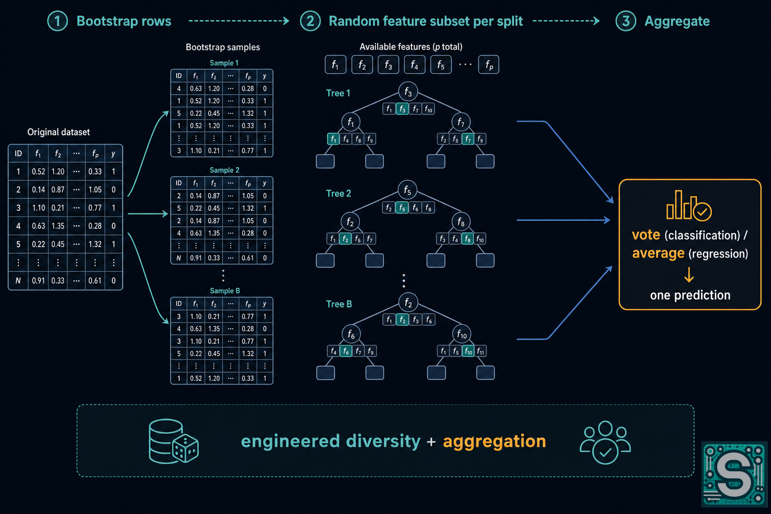
Random forests aggregate in a very direct way:
For classification, each tree outputs a class label, and the forest predicts the class with the most votes (sometimes using predicted probabilities and averaging those).
For regression, each tree outputs a numeric value, and the forest predicts the average of those values.
If you pause and reflect, both are doing the same conceptual thing: they are dampening the influence of any single tree’s overconfident, idiosyncratic judgment.
A deep decision tree can be extremely certain in tiny regions of the feature space, because its leaves may be defined by a long chain of splits that isolate only a few training points. If one of those points is a fluke, the leaf’s prediction can be wildly off - but the tree will still commit to it. When you average across many trees, those extreme leaf-level quirks tend not to align. One tree’s “this house is definitely worth $1.2M” gets balanced by another tree’s “I’ve never seen this pattern; I’m closer to $850k”. The forest ends up less jumpy.
It’s also helpful to see the voting effect numerically in a small, reproducible example.
Worked example: majority vote can amplify correctness
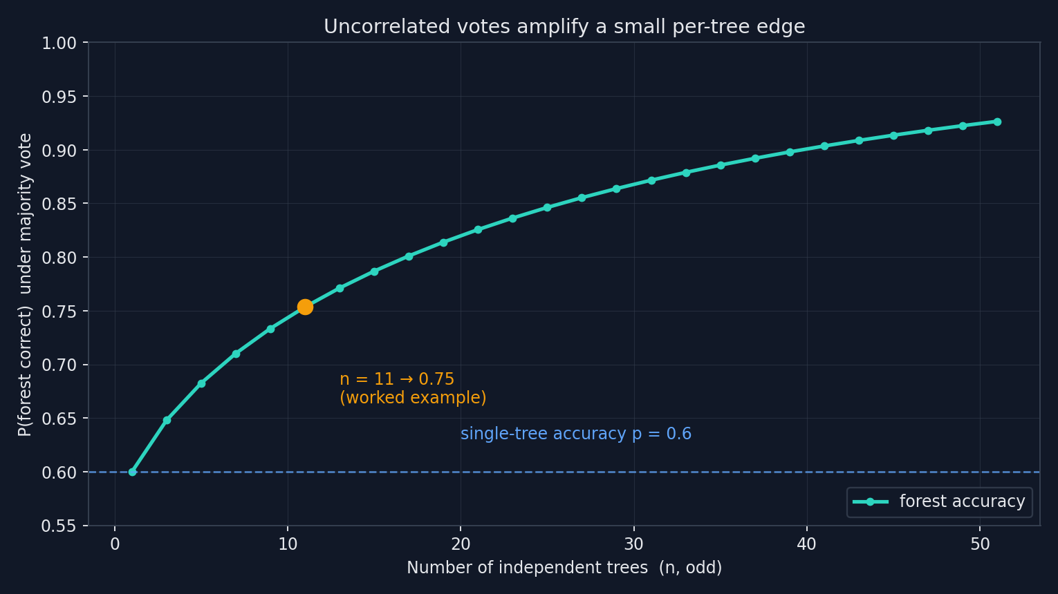
Assume a binary classification task. Suppose each tree is correct with probability p, and (to keep the math simple) the trees’ errors are independent. Let n=11 trees, and let K be the number of trees that vote correctly. Then:
The forest is correct if a majority votes correctly, i.e. K≥ 6.
Take p=0.6. Then:
Let q=1-p=0.4. Now compute each term:
k=6: C(11, 6)=462,0.6⁶=0.046656,0.4⁵=0.01024, Term=462·0.046656·0.01024≈ 0.2207k=7: C(11, 7)=330,0.6⁷=0.0279936,0.4⁴=0.0256, Term≈ 0.2365k=8: C(11, 8)=165,0.6⁸=0.01679616,0.4³=0.064, Term≈ 0.1774k=9: C(11, 9)=55,0.6⁹=0.010077696,0.4²=0.16, Term≈ 0.0887k=10: C(11, 10)=11,0.6¹⁰=0.0060466176,0.4¹=0.4, Term≈ 0.0266k=11: C(11, 11)=1,0.6¹¹=0.00362797056, Term≈ 0.0036
Sum them:
So we went from a single-tree accuracy of 0.6 to a forest accuracy of about 0.75, because the errors weren’t aligned. If the trees were highly correlated, this gain would shrink - again reinforcing that sameness is the real problem.
A concrete story: predicting house prices with many imperfect rules
Let’s tell a story rather than do more math.
Suppose you’re predicting house prices. Your dataset includes square footage, number of bedrooms, age, a neighborhood label, distance to downtown, school rating, and maybe a few messy proxies like “has renovated kitchen” extracted from listings.
A single decision tree might do something like this: it notices that in the training data, houses labeled “Neighborhood A” are expensive. Maybe that neighborhood label is genuinely meaningful. Or maybe you scraped data during a period when only high-end listings from Neighborhood A were active, or perhaps the label is inconsistently applied by agents. The tree doesn’t know any of that. It just sees a feature that reduces error quickly, so it splits early on neighborhood and commits.
Downstream, it adds more rules. If Neighborhood A and square footage above 2000, predict $1.1M. If Neighborhood A and square footage below 2000 but renovated kitchen, predict $950k. Soon the leaves become very specific. And because the tree is deep, it can create tiny regions that look extremely “pure” in the training set.
Now imagine you build a forest.
One tree’s bootstrap sample happens to include more mid-range Neighborhood A homes. That tree decides neighborhood is less decisive and splits first on square footage. Another tree’s feature subset at the root doesn’t even include neighborhood, so it splits on distance to downtown. A third tree splits on school rating. A fourth tree does use neighborhood early, but later splits differ because it sees a slightly different mix of examples.
So when you feed in a new house - say, a 1900 sq ft home in Neighborhood A with a renovated kitchen - the forest produces a set of opinions. Some trees anchored on neighborhood might still go high. Others anchored on size and distance might be more conservative. The average ends up reflecting a broader set of patterns: it’s less likely to be dominated by one brittle rule like “Neighborhood A implies luxury”, because not every tree was allowed to build that same story.
This is the “calmness” random forests are famous for in tabular data. They’re not magic; they’re a system that makes it harder for any single coincidence to become the whole explanation.
What “weak” really means here (and what it doesn’t)
It’s easy to get confused by ensemble vocabulary, especially if you’ve heard phrases like “weak learners” in boosting.
In random forests, the individual trees are often not weak in the sense of being shallow or simplistic. In fact, many random forest implementations grow trees quite deep - sometimes until leaves are small or pure, unless you explicitly stop them with parameters like maximum depth or minimum leaf size.
So why do people talk about weakness at all?
Because each tree is trained under conditions that make it noisy:
It sees a bootstrap-resampled dataset, so it may miss some important examples and over-see others.
At each split, it may be forced to choose among a limited subset of features, which can push it toward a “pretty good” split rather than the globally best one.
If trees are allowed to grow deep, they can memorize peculiarities of their own resampled data.
A single such tree might be a strange character: confident, specific, and occasionally very wrong. It’s “weak” not because it lacks capacity, but because it’s not trained to be a stable, globally optimal predictor. It’s trained to be one member of a crowd.
This is a subtle but important mental shift. In many ML problems, you try to train one model that is as good as possible given the data. With random forests, you’re intentionally creating a distribution of models - a set of perspectives - so that aggregation does the stabilizing work.
The strength is in the system design: the forest uses high-capacity components (trees) but arranges them so that their high variance becomes a resource rather than a liability. That design only pays off when you preserve diversity and then combine predictions in a way that cancels idiosyncrasies.
When the crowd fails: limits and trade-offs you should expect
Random forests are often a strong default for tabular data, but they’re not a free lunch. The “wisdom of the crowd” metaphor is useful here too, because real crowds have costs and failure modes.
First, forests can be heavier than a single tree. Training involves building many trees, and inference involves running a new example through all of them. If you have hundreds or thousands of trees and strict latency constraints, this can matter. In practice, forests are often still quite usable - but the cost is real, and you should measure it rather than assume it’s negligible.
Second, you give up interpretability. A single decision tree can be read like a flowchart. You can audit it, argue with it, and sometimes present it to non-technical stakeholders. A forest is a committee. You can inspect individual trees, but the final decision is not “one path”. It’s an aggregate of many paths, and that’s harder to narrate honestly.
Third, random forests do not solve dataset shift or missing signal. If your training data does not represent the deployment environment, a forest will confidently generalize the wrong lessons - just more stably. Similarly, if the signal is extremely subtle relative to noise, diversity cannot invent information. The crowd can cancel noise; it cannot conjure a pattern that isn’t encoded in the features.
Finally, forests can struggle in settings where structure matters more than tabular heuristics - think high-dimensional sparse text, images, or problems where smooth, differentiable representation learning is the right tool. You can use forests there, but you’re often fighting the problem’s geometry.
The right expectation is: random forests are a dependable, pragmatic method for many supervised learning tasks, especially on structured data - but they inherit the limitations of “learning from examples” and add computational and interpretability costs.
The “more trees is always better” myth
There’s a common instinct when you first learn about random forests: if 100 trees are good, 1000 must be better, and 10,000 must be amazing.
The truth is more nuanced, and it mirrors the earlier variance math.
As you add trees, the forest’s predictions usually become more stable. In regression, the averaged prediction variance tends to decrease; in classification, the vote becomes less sensitive to any one tree’s quirks. But this improvement has diminishing returns. After some point, each additional tree mostly agrees with the existing crowd, and you’re paying extra computation to shave off tiny fluctuations.
Two practical realities show up:
Validation performance plateaus. You’ll often see accuracy (or RMSE, or AUC) improve quickly from, say, 10 to 100 trees, improve a bit more from 100 to 300, and then barely move after that. The exact numbers depend on your dataset, but the shape of the curve is common.
Inference cost is linear in the number of trees. Doubling trees doubles the number of tree traversals per prediction. If you care about latency or throughput, you can’t ignore this.
A good habit is to treat n_estimators (number of trees) as primarily a stability knob. Add trees until your validation metric is stable and your latency budget is still happy. If you have plenty of compute and you want maximum performance, sure - push it further. But do it with measurement, not faith.
One subtle point: if your trees are too correlated (for example, because your feature randomness is too low or your data is very dominant along one feature), adding more trees may plateau even earlier. In that case the fix is often not “more trees”, but “less sameness”.
The “feature importance” trap: what the forest can and can’t explain
People love asking random forests what they “learned”, and feature importance is the most common way this shows up. Most libraries will give you some measure of importance - often based on how much each feature reduces impurity across splits, or based on how much shuffling a feature hurts performance.
These signals can be genuinely helpful. If a feature consistently matters across many trees, that often indicates it’s predictive. In messy real-world datasets, feature importance can guide debugging: “Why is this ID-like feature so important?” can reveal leakage. Or it can guide product thinking: “Are we actually using the expensive-to-collect feature, or is it redundant?”
But it’s easy to over-read these numbers, because a forest is not a causal model. It’s an opportunistic predictor.
Two common traps:
Correlated features share credit in weird ways. If two features are strongly correlated (say, “square footage” and “number of bedrooms”), the forest can split on either one. Importance may concentrate on whichever feature happened to win splits more often, even if both encode similar signal. This doesn’t mean the other feature “doesn’t matter”; it may simply be redundant.
Dataset quirks can look like meaning. If a feature is a proxy for how the data was collected (timestamp, region code tied to a particular marketing campaign, source system identifier), the forest might use it heavily. Importance then reflects your pipeline, not the world.
The most grounded way to think about it is: a random forest is a strong predictor first, and only a partial explainer in context-dependent ways. Use feature importance to ask better questions, not to conclude a story about why outcomes happen.
Tuning without superstition: the knobs that change the forest’s personality
Hyperparameter tuning for random forests can feel like folklore: “use 500 trees”, “depth doesn’t matter”, “always set max features to sqrt”. There are reasons those heuristics exist, but you’ll get much further if you map each knob to the problem it’s trying to solve.
Number of trees (`n_estimators`). This mostly controls variance reduction through averaging. More trees makes the forest’s output less sensitive to the randomness in bootstrapping and feature subsets. Past a point, returns diminish, so it’s a stability-versus-cost trade.
Tree depth / leaf size (`max_depth`, `min_samples_leaf`). This controls how much each tree can memorize its bootstrap sample. Deep trees with tiny leaves can fit idiosyncrasies; that’s not automatically bad in a forest, but if leaves are too small, each tree becomes extremely noisy. Increasing min_samples_leaf forces smoother rules: leaves represent broader regions, which often improves generalization.
Features per split (`max_features`). This is one of the most “personality-changing” knobs because it directly affects diversity. If max_features is large, many trees will repeatedly choose the same strong predictors early, increasing correlation. If it’s small, trees are forced into different early narratives, which can reduce correlation - but if it’s too small, trees may become weak in the unhelpful sense of missing important signal at many splits.
Bootstrap / sampling choices. Bootstrapping is a built-in way to perturb the training set. If you turn it off (or if your dataset is tiny), trees may become more similar. Conversely, with enough data, bootstrapping can be a gentle way to create diversity without losing too much signal.
A good tuning mindset is: pick a validation metric you trust, tune toward lower error and manageable cost, and interpret each change as “I’m trading off memorization, diversity, and stability”.
💬 What did a random forest once teach you the hard way - a feature-importance trap, a leakage surprise, a plateau that “more trees“ couldn’t fix? I read every reply.
Zooming out: what random forests teach you about machine learning
If you step back, random forests are less about trees and more about a philosophy of building reliable systems from unreliable parts.
Early in ML, it’s natural to search for the “right model” - the one that captures the true structure of the data. That’s an understandable instinct, and sometimes it works. But many real datasets don’t reward a single pristine story. They’re messy: measurement error, hidden confounders, shifting distributions, proxies standing in for unmeasured variables, and feedback loops from the very systems we build.
In that world, brittleness is the default. A model that depends on one fragile narrative - one feature behaving “the same way forever”, one clean separation that only exists in your snapshot of data - will eventually surprise you.
Random forests embody a different approach: design for resilience. Encourage multiple perspectives. Prevent any one strong but possibly misleading predictor from dominating every decision. And then aggregate in a way that rewards consistent signal and penalizes idiosyncratic noise.
This is a lesson you can carry beyond random forests. It shows up in cross-validation, in regularization, in ensembling across model families, in monitoring and drift detection, and even in engineering practices like canary deployments. We don’t just want models that can fit. We want models (and systems) that behave sensibly when the world wiggles.
A random forest, at its best, is a structured way to turn disagreement into reliability. Not because disagreement is intrinsically good, but because it’s evidence that you’re not trapped in one overconfident story. And in machine learning - where the world is always a bit more complicated than our datasets - that humility is often the most practical form of intelligence.
📬 This is Machine Learning Fundamentals - one method, built up from intuition to the math that makes it work, no hype. Subscribe and the next one lands in your inbox.
References
Ensemble methods: forests of randomized trees | scikit-learn
Random Forests by Leo Breiman | Machine Learning (2001)
XGBoost: A Scalable Tree Boosting System by Tianqi Chen & Carlos Guestrin | arXiv
An Introduction to Statistical Learning by James, Witten, Hastie & Tibshirani | Springer (free online)
The Elements of Statistical Learning by Hastie, Tibshirani & Friedman | Stanford (free online)
Pattern Recognition and Machine Learning by Christopher Bishop | Microsoft Research (free PDF)
Classification and Regression Trees by Breiman, Friedman, Olshen & Stone | Chapman & Hall
 |
|