
Logistic Regression — when machines learn to say yes or no
Machine learning fundamentals


⚠️ Before we begin — a practical AI newsletter worth following

GenAI Unplugged by Dheeraj Sharma focuses on building simple AI automation systems for solopreneurs. Instead of abstract AI discussions, you’ll find step-by-step guides for creating agents, automating workflows, and turning repetitive work into systems that actually save time.
Binary classification sounds crisp: yes or no, spam or not spam, churn or stay. But most real decisions don’t feel crisp at all. They feel like standing in fog with a flashlight: you can see some evidence, but not enough to feel certain.
Think about a simple question a product team might ask: “Will this package arrive late?” There’s a tracking history, a carrier, a destination, weather, time of year, warehouse load. You don’t look at those signals and instantly “know” the answer. What you actually form is a belief - an internal probability. Probably late. Maybe on time. And only after that belief forms do you decide what to do: proactively message the customer, offer a discount, or do nothing.
Logistic regression is the machine learning version of that habit. It does not begin by trying to shout “YES” or “NO”. It begins by learning how to weigh evidence and turn that evidence into a probability. The “classification” part - the conversion from probability to a label - comes later, and (crucially) it is not a law of nature. It’s a choice you make based on costs, risk tolerance, and what kind of mistakes your system can live with.
This post is a slow walk through that mental model. We’ll build logistic regression from the inside out: an evidence score, a squashing function, a probability, and then an optional decision rule. We’ll derive the loss function step by step (no “it can be shown”), and we’ll do small numeric examples you can reproduce with a calculator. If you’ve ever felt that logistic regression was “just a formula”, the goal here is to make it feel like a clear, reasonable machine for turning messy signals into honest odds.
A yes-or-no question rarely feels like yes-or-no
Imagine you run a subscription app and you’re looking at a particular user. The question on your dashboard reads: “Will this customer churn in the next 30 days?” That is technically a binary question. Either they will, or they won’t.
But your experience of the question isn’t binary. You don’t think in labels first. You think in likelihoods: They haven’t logged in for two weeks… that’s bad. But they just upgraded… that’s good. They contacted support twice… unclear. Your brain starts doing an informal accounting of evidence, and the output is rarely a hard label. It’s something like: “I’m worried. Maybe 70%”.
That “odds-first” habit is not a weakness; it’s often the most rational way to behave under uncertainty. If an action is expensive (a retention phone call), you might require high confidence. If an action is cheap (an automated helpful email), you might act on weaker suspicion.
Logistic regression fits neatly into this worldview. It aims to learn a mapping from features (signals) to a probability like 0.72, not directly to a label. It learns how strongly each signal should influence the belief, using past data as feedback.
A subtle point that matters later: the model’s probability is not a statement about a single individual’s soul. It’s a statement about frequency in similar cases. If the model outputs 0.7 on many users, you want roughly 70% of those users (in that slice of feature space) to actually churn. That’s the core: treat binary outcomes as probabilistic events with learnable structure.
🔎 Ever wondered how machines actually decide “yes” or “no”?
If you enjoy breaking down machine learning ideas into clear intuition instead of heavy math, you’ll probably like the rest of this series. Subscribe 👇
Why probabilities are often more useful than labels
If you force every prediction into a hard 0 or 1, you throw away information that could have driven better decisions.
Consider two churn predictions:
User
A: (p = 0.51)User
B: (p = 0.99)
If you use a default threshold of 0.5, both become “yes: will churn”. But treating these users identically is usually irrational. User A is barely over the line - almost a coin flip. User B is practically screaming.
In real systems, this difference affects:
Resource allocation. A retention team might have time to call only the riskiest users. You want to sort by probability, not by label.
Human review. Borderline cases are perfect for a queue, where a person can decide with extra context.
User experience. You might show a gentle in-app nudge at
0.6, but a stronger offer at0.95.Cost-sensitive decisions. If false positives are expensive, you may require a higher probability before acting.
Probabilities also let you talk about performance in a richer way. Accuracy collapses everything into “right or wrong”, but probabilities support calibration curves, expected cost calculations, and ranking metrics. A model that says 0.6 for everything might get some labels right, but it’s not useful in the same way a well-shaped probability model is.
So the goal is not merely to “classify”. The goal is to produce a probability that is as honest as possible - meaning: aligned with reality across many examples. Logistic regression is one of the simplest models that tries to do exactly that, and its simplicity is part of why it’s still worth learning deeply.
The model’s inner voice: “How much evidence points to yes?”
Before we name anything, let’s build the mental picture.
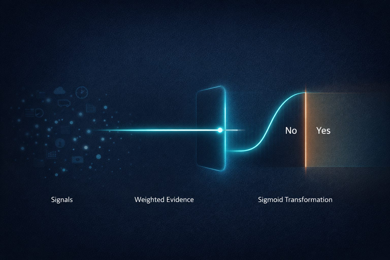
Logistic regression creates a single number - a kind of internal “evidence score”. Each feature contributes a push:
Some features push the score upward (more evidence for “yes”).
Others push it downward (more evidence for “no”).
The pushes add together.
This is very close to how you might make a decision with a checklist. “Late delivery risk” might increase if it’s winter, if the destination is far, if the carrier is overloaded. Those are pushes. You add them up into an overall sense of risk.
Mathematically, this “weighted checklist” is a linear combination. Suppose your features are:
The model learns weights:
And it also learns a baseline offset (often called an intercept):
The evidence score is:
That’s the whole inner voice: a sum of nudges. If (wᵢ) is positive, higher (xᵢ) pushes toward “yes”. If (wᵢ) is negative, higher (xᵢ) pushes toward “no”.

Worked example: computing an evidence score
Problem. Compute the evidence score (z).
Given.
(b = -1.2)(w₁ = 0.8), (x₁ = 2.0)(w₂ = -0.5), (x₂ = 1.0)(w₃ = 0.3), (x₃ = 4.0)
Step 1: compute each push.
Step 2: add them with the intercept.
Meaning. The model’s internal evidence is positive ((z = 1.1)), so it is leaning toward “yes”. But we still don’t have a probability - yet.
The squashing step that turns evidence into a probability
An evidence score like (z) can be any real number: (-10), (1.1), (200). But a probability must live between 0 and 1. So we need a function that converts an unbounded score into a bounded probability.
Even before we name the function, we can describe what we want:
Very negative evidence should map to a probability near
0.Very positive evidence should map to a probability near
1.Evidence near
0should map to something like “uncertain”, around0.5.The mapping should be smooth, not a hard step, because small evidence changes shouldn’t cause discontinuous probability jumps.
The classic choice is the sigmoid (also called the logistic function). It’s defined as:
And logistic regression uses:
where (p) is the predicted probability of the positive class (“yes”).

Why this shape? One intuitive way to see it is to look at extremes:
If (z) is very large and positive, then (-z) is very negative, so (e⁻ᶻ) is near 0. Then:
If (z) is very large and negative, then (-z) is very positive, so (e⁻ᶻ) is huge. Then the denominator is huge, and (p) is near 0.
At (z = 0):
So zero evidence corresponds to 50/50 odds. And the curve is S-shaped: slow at the ends, fast in the middle. That “fast in the middle” turns out to be where most of the learning action lives.
💡 Did this visualization make logistic regression finally click?
Sometimes a single diagram explains what pages of equations cannot.
💬 Leave a comment - I’m curious what part made the idea clearer for you.
Worked example: from evidence to probability
Problem. Convert (z = 1.1) into a probability.
Given. (z = 1.1)
Step 1: compute (e⁻ᶻ).
Step 2: compute the denominator.
Step 3: invert.
Meaning. Evidence score (1.1) corresponds to about a 75% predicted chance of “yes”. Notice how that feels: a positive lean, not absolute certainty.
Why the middle matters: uncertainty lives near the boundary
The sigmoid’s most important region is not near 0 or near 1. It’s the middle.
When (z) is very large (say (z = 8)), the sigmoid is already extremely close to 1. Changing (z) a little doesn’t change the probability much:
(z = 8 ⇒ p ≈ 0.9997)(z = 7 ⇒ p ≈ 0.9991)
Those are different numbers, but they are operationally similar: high confidence “yes”.
In contrast, near (z = 0), small changes move the probability a lot:
(z = 0 ⇒ p = 0.5)(z = 0.4 ⇒ p ≈ 0.598)(z = -0.4 ⇒ p ≈ 0.401)
This region corresponds to borderline cases - users who might churn or might not, emails that look a bit spammy but not definitely spam, transactions that are suspicious but plausibly legitimate.
Two things make the middle region special:
During training, these examples carry a lot of information. If the model is uncertain but wrong, it needs to adjust weights so similar cases move the correct direction. If the model is already extremely confident and correct, there’s not much to learn from that point.
During deployment, these examples are the risky ones. A slight shift in the real world (seasonality, new user behavior, a policy change) can push many borderline cases across your chosen threshold, causing visible behavior changes.
If you remember only one operational lesson: pay attention to the probability mass near your decision boundary. That’s where your metrics will be sensitive, where calibration matters, and where product decisions about thresholds will show up as real outcomes.
From probability to decision: the threshold is not part of the truth
Logistic regression outputs a probability (p). That’s the model’s belief.
A decision rule is something you add on top:
Here (t) is the threshold you choose.
It’s tempting to treat (t = 0.5) as “the default”, almost like physics. But it’s not physics. It’s values.
To see why, imagine two scenarios:
Medical screening. A test flags “possible disease”. Missing a true case (false negative) might be very costly. You might set (t) low, perhaps 0.2, accepting more false alarms in exchange for catching more true positives. The follow-up test might be cheap and safe, so false positives are tolerable.
Account bans for fraud. Now a false positive is a serious accusation that harms a user. You might set (t) high, maybe 0.95, accepting that you will miss some fraud in exchange for avoiding wrongful bans.

In both cases, the same predicted probability can lead to a different action. That’s not inconsistency; it’s a separation of responsibilities:
The model estimates probabilities as honestly as it can.
The system chooses actions based on costs and risk tolerance.
Worked example: choosing a threshold by expected cost
Problem. Pick the cheaper action using expected cost.
Given.
Model outputs
(p = 0.30)for “fraud”.Cost of blocking a legitimate user:
(CFP= 50)Cost of letting fraud through:
(CFN= 10)
If we block, we pay (50) only if it’s not fraud, which happens with probability (1 - p).
If we allow, we pay (10) only if it is fraud, which happens with probability (p).
Decision. Allow is much cheaper in expectation (3 vs 35). Even though 30% fraud risk sounds scary, the action costs dominate the choice. This is the kind of reasoning probabilities enable - and hard labels destroy.
A grounded example: churn prediction as a weighted checklist
Let’s make this concrete with a small churn story. Suppose we run a subscription app and define “churn” as canceling within 30 days. We build features for each user:
(x₁):days since last login(x₂):number of support tickets in last 30 days(x₃):discount usage (0 or 1)(x₄):plan type (0 for annual, 1 for monthly)
We train logistic regression and get weights (these are fictional but plausible):
(b = -2.0)(w₁ = 0.12)(w₂ = 0.40)(w3= 0.90)(w4= 0.70)
Interpretation: more days since login increases churn risk; more support tickets increases churn risk; using discounts is a risk signal (maybe bargain-seekers churn); monthly plans churn more than annual.
Now compare two users.
User A (mild risk)
days since login:
(x₁ = 8)support tickets:
(x₂ = 1)used discount:
(x3= 0)monthly plan:
(x4= 1)
Evidence score:
Compute pushes:
Sum:
Probability:
User A is barely above 50/50: “keep an eye on them”.
User B (high risk)
days since login:
(x₁ = 20)support tickets:
(x₂ = 3)used discount:
(x3= 1)monthly plan:
(x4= 1)
Evidence:
Compute pushes:
Sum:
Probability:
Now we have two “likely churn” users, but one is ~0.52 and the other is ~0.96. In a real retention workflow, User A might get a gentle reminder email. User B might justify a retention call or a targeted offer. The power here is not the label; it’s the ranked, calibrated belief.
What training is actually doing: adjusting how much each signal counts
So far we’ve treated the weights as magic numbers we somehow obtained. Training is the process of choosing those weights so that the predicted probabilities match reality well across many examples.
Let’s formalize one data point. For user (n):
features:
(x⁽ⁿ⁾)label:
(y⁽ⁿ⁾ ∈ 0, 1)
predicted probability:
[ p⁽ⁿ⁾ = σ(z⁽ⁿ⁾) ]evidence score:
[ z⁽ⁿ⁾ = b + wᵀx⁽ⁿ⁾ ]
Now: how should a model be rewarded or punished? Intuitively:
If the true label is
1and the model says(p = 0.99), that’s great.If the true label is
1and the model says(p = 0.51), that’s only mildly good.If the true label is
1and the model says(p = 0.01), that’s disastrously overconfident and should hurt a lot.
This “confidently wrong should hurt more” idea leads to log loss (also called cross-entropy for binary classification). Here’s the clean derivation from probability, not from tradition.

Step-by-step derivation from a Bernoulli likelihood
For a binary outcome (y), if the model predicts probability (p) of (y = 1), then the probability of observing (y) is:
If
(y = 1):probability is(p)If
(y = 0):probability is(1 - p)
We can write both cases in one expression:
Now training wants to choose parameters that make observed labels likely. That means maximizing the likelihood over all data points, or equivalently maximizing the log-likelihood (log is monotonic and turns products into sums).
For one example:
Use log rules:
To turn this into a loss we minimize, we negate it:
That is the binary log loss.
Notice what it does: if (y = 1), the loss is (-log(p)), which goes to infinity as (p ➝ 0). That’s the “confidently wrong hurts a lot” property, mathematically enforced.
Worked example: log loss for two predictions
Problem. Compare losses for a correct-but-uncertain prediction and a correct-and-confident one.
Given. True label (y = 1). Two predictions: (p₁ = 0.6), (p₂ = 0.95).
When (y = 1), loss is:
For (p₁ = 0.6):
For (p₂ = 0.95):
Meaning. Both are “correct” under a 0.5 threshold, but the confident correct prediction is rewarded much more (smaller loss). Training with this loss nudges the model to be not just correct, but calibrated and decisive when the evidence supports it.
Reading the model: coefficients as directional pushes (with caveats)
One of logistic regression’s most attractive traits is that it’s interpretable in a very practical sense. If you look at the learned coefficients:
A positive
(wᵢ)means feature(xᵢ)pushes probability toward “yes”.A negative
(wᵢ)means it pushes toward “no”.Larger magnitude generally means a stronger push.
There’s also a deeper and very useful interpretation that connects directly to the evidence score. Logistic regression makes the evidence score linear:
And then:
Because the sigmoid is monotonic, increasing (z) always increases (p). So coefficients literally control the direction of probability movement.
You will also hear a statement like: “coefficients correspond to log-odds”. That can be made explicit by solving the sigmoid for (z).
Start from:
Invert both sides:
Subtract 1:
Combine terms:
Take log:
Multiply by (-1):
So the evidence score (z) is the log-odds. Each feature contribution (wᵢ xᵢ) is a contribution to log-odds.
Now, the two gotchas that surprise beginners:
Gotcha 1: feature scale matters. If one feature is measured in days (0–365) and another is a binary flag (0/1), the day feature can have a small coefficient and still dominate the sum. Comparing raw coefficient magnitudes without standardizing features can be misleading.
Gotcha 2: correlated features share credit. If two features are strongly correlated (say “days since last login” and “number of sessions last month”), the model can distribute weight between them in many equivalent ways. Individual coefficients may look unstable across retraining runs, even when predictions remain stable. Interpret coefficients with care: they are not always “causal importance”.
What logistic regression can and cannot represent
Logistic regression draws a boundary that is linear in feature space (or, said differently, it separates examples using a hyperplane in the original feature space). The probability changes smoothly as you move across that boundary.
That structure is a strength. It means:
Fast training. You can fit large datasets efficiently.
Robustness. With regularization, it tends not to overfit wildly.
A strong baseline. If you can’t beat logistic regression, you often don’t yet understand the problem or the features.
Reasonable extrapolation. Linear evidence behaves predictably outside the training set (though not always correctly).
But it is also a limitation. If the true relationship between features and outcome is highly non-linear - say, churn risk spikes only for a specific combination of behaviors, or fraud looks like a complicated “island” in feature space - then a single linear boundary may not capture it well.
There’s an important nuance: logistic regression is linear in the features you give it, not necessarily linear in the raw world. You can engineer features that expose non-linear structure. For example:
Add polynomial terms like
(x²)Add interactions like
(x₁ x₂)Use splines or bucketed features
Once you add those engineered features, logistic regression can represent more complex boundaries - but you paid for that complexity by choosing the right transformations.
In practice, this is why logistic regression often shines in domains with well-designed features (ads, ranking, many tabular problems). It’s not glamorous. It’s just honest about what it can represent: a smooth ramp from “no” to “yes” driven by additive evidence.
When it fails in real systems: rare events, noisy labels, drifting populations
Most textbook explanations end when the model is trained. Real problems start after deployment.
Rare events. In fraud, serious adverse events, or rare diseases, positives may be 0.1% of the data. A logistic regression model can still output probabilities, but those probabilities can be poorly grounded if you evaluate incorrectly or if the model is pushed into regions with little positive data. You may see confident-looking numbers that are driven more by class imbalance and feature quirks than by true signal. Handling this often requires careful sampling strategies, appropriate metrics (like precision-recall curves), and explicit attention to calibration.
Noisy labels. Suppose “churn” is defined as “no activity for 30 days”, but many users are seasonal and return later. Now your labels encode ambiguity. Logistic regression will respond by pushing probabilities toward the middle because the same feature patterns sometimes map to 1 and sometimes to 0. That is not the model being “weak”; it is the model reflecting inconsistency in the target definition. If your organization expects crisp predictions from fuzzy labels, you will fight endlessly.
Drifting populations. The most insidious failure is distribution shift. The model is trained on last year’s user behavior, but this year you introduced a new onboarding flow, a new pricing tier, or a competitor launched something disruptive. Now the relationship between features and churn changes. Your “0.8” probabilities may stop meaning “80%”. They might behave like “60%” in today’s world. That’s a calibration break caused by a moving target.
Operationally, this is why monitoring matters: not just accuracy, but calibration, feature distributions, and decision outcomes. Logistic regression is simple, but the system around it is not. The model’s humility - expressed as a probability - can be lost if you treat it like a deterministic oracle.
Misunderstandings worth clearing up early
A few confusions come up so often that it’s worth clearing them early, before they calcify into mental bugs.
“Why is it called regression if it’s classification?” Historically, “regression” refers to modeling a numerical quantity. Logistic regression models a numerical quantity: the probability (P(y=1|x)). The output is continuous. We then optionally threshold it to get a class label. So the name is less wrong than it sounds; it’s just anchored in the probability-first view rather than the label-first view.
“If the model says 0.9, does it know the answer?” No. A probability is not a promise about this individual case. It’s a statement about frequency among similar cases. If the model is well-calibrated, then among all cases where it predicts 0.9, about 90% should be positive. That’s a population-level claim, not a metaphysical certainty about one example.
“Is 0.5 the default threshold?” It’s a default in the sense that it’s a convenient midpoint, but it’s rarely the right choice automatically. If false positives and false negatives have different costs (they almost always do), the optimal threshold can be far from 0.5.
“Does logistic regression output ‘real probabilities’?” It outputs numbers between 0 and 1 that are trained using a probability-based loss. Whether those numbers behave like real-world probabilities depends on calibration, data quality, and whether the deployment distribution matches training. Logistic regression is often reasonably calibrated compared to some more flexible models, but there are plenty of ways it can be miscalibrated in practice.
If you keep the probability-first mental model, these misunderstandings mostly dissolve. Confusion tends to enter when we treat the label as truth and the probability as a decoration, rather than the other way around.
🚀 Know someone who still finds logistic regression confusing?
A simple mental model often helps more than another textbook explanation.
🔁 Share this post with someone learning machine learning.
Closing reflection: a small model with a big lesson
Logistic regression is often introduced as a “baseline classifier”, which is technically true and psychologically unfair. It’s more than a baseline. It’s one of the cleanest examples of a principle that scales all the way up to modern machine learning systems:
Separate belief from action.
The model’s job is belief: given evidence, output an honest probability. Your system’s job is action: choose what to do given that belief, your costs, your risks, and your values. When you blur these two roles - when you treat a probability as a label, or a threshold as truth - you lose control. You also lose the ability to have clear conversations with stakeholders about trade-offs, because everything collapses into “the model said so”.
Logistic regression also teaches a quieter lesson about mathematics in ML: the formulas are not arbitrary. The sigmoid is not a random squashing function; it is a convenient, interpretable bridge between additive evidence (log-odds) and probabilities. Log loss is not a punishment invented to scare you; it falls directly out of maximum likelihood for a Bernoulli outcome, and it encodes a very human idea: confident wrongness should hurt.
If you later move to gradient-boosted trees, neural nets, or large language models, this framing still helps. You can ask: what is the model’s belief representation, how is it trained to be honest, and where do we convert beliefs into decisions? Logistic regression is small enough to fit in your head, but big enough to teach that habit well.
The Elements of Statistical Learning: Data Mining, Inference, and Prediction, Second Edition by Trevor Hastie, Robert Tibshirani, Jerome Friedman
Machine Learning: A Probabilistic Perspective (Adaptive Computation and Machine Learning series) by Kevin P. Murphy
Pattern Recognition and Machine Learning (Information Science and Statistics)
by Christopher M. Bishop
Information Theory, Inference and Learning Algorithms by David J. C. MacKay
Stanford CS229 notes (linear regression + optimization) by Andrew Ng and Tengyu Ma
scikit-learn documentation for
LogisticRegression