
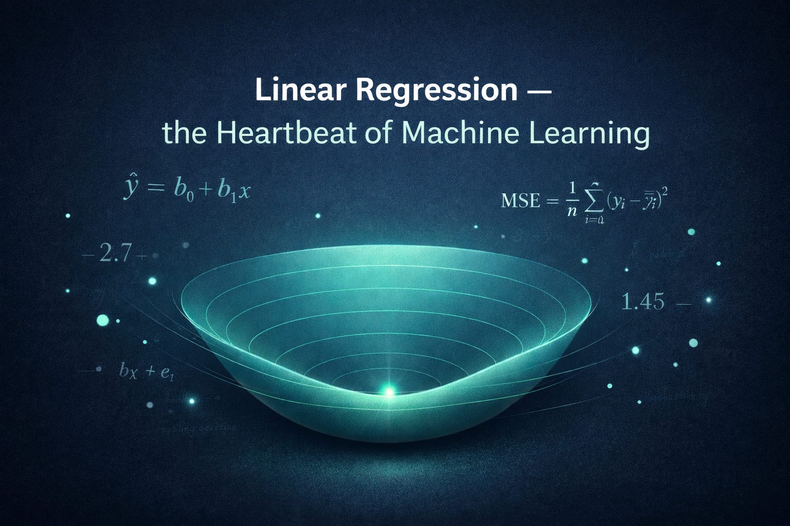
Linear Regression — the heartbeat of Machine Learning
Machine learning fundamentals

Linear regression looks almost trivial on the surface: you draw a straight line through a cloud of points and use it to predict (y) from (x). But that “almost” hides why it has survived for so long. Linear regression is the first model where you can see - clearly, concretely - the full learning loop that powers much of machine learning: propose a parameterized rule, measure its failures, and change the parameters to reduce those failures.
In other words, linear regression isn’t memorable because lines are special. It’s memorable because it’s the simplest place where optimization becomes a way of thinking. You’re not trying to “be right”. You’re trying to be less wrong according to a score you chose on purpose. That’s an idea you will reuse everywhere: logistic regression, matrix factorization, gradient-boosted trees, neural networks, language models. The shapes change, the data changes, the number of parameters explodes - but the heartbeat is recognizable.
This post is deliberately slow. I’m going to spend time on the emotional problem (“the world is messy and I still want a simple story”), then the modeling decision (“a line is a constraint we choose”), and only then the mechanics (“how do we adjust the knobs?”). When we do introduce math, we’ll treat it like a guided walkthrough, not a magic incantation. The goal is that you could sit down with a notebook and re-derive the essentials yourself - and, more importantly, that you’ll know what to look for when the line inevitably fails.
The comforting lie of a clean relationship
Most of us begin modeling with a quiet hope: more of X means more of Y. It’s a reasonable hope because it’s often directionally true. More practice tends to improve performance. More advertising tends to increase sales. More weight on a spring tends to stretch it further. These are comforting because they offer a simple story you can tell yourself and others.
Then you actually plot the data.
Instead of a neat diagonal trend, you get dots that wobble. They clump. They contradict each other. You might see points with high (x) and low (y), and low (x) and high (y), all in the same dataset. If you were expecting a clean relationship, the scatter plot feels like a betrayal: “Was my intuition wrong? Is there no relationship at all?”
This is the emotional problem linear regression solves. Not “how do I find the truth”, but: how do I tell a simple story about a messy world in a way that can be defended? The defensible part is crucial. Anyone can eyeball a plot and draw a line they like. But two people will draw two different lines. If your story depends on taste, you haven’t learned anything stable.
Linear regression offers a truce. It says: we will accept that points do not line up perfectly, and we will still insist on a simple summary - but we will choose that summary according to a clear rule. Not because the rule is perfect, but because it is explicit, repeatable, and critique-able. That is what turns a comforting lie into an engineering tool.
Drawing a line is really choosing a kind of explanation
A straight line is not “the default” because reality is linear. It’s the default because it is the simplest explanation that can still be wrong in a useful way. That sounds almost philosophical, but it’s practical: if you allow yourself to fit anything - curves, kinks, weird oscillations - you can always build a model that matches the data you already saw. The hard part is building something that will behave sensibly on data you haven’t seen.
A line is a bias toward simplicity. It says: “I will explain the relationship using only two degrees of freedom: an overall vertical shift and a tilt”. That constraint is what makes a line interpretable. You can point at it and say something like: “For every additional unit of (x), the predicted (y) changes by a constant amount”. That is a statement a human can reason about.
This is a general pattern in machine learning: we choose a family of explanations, then search within that family. Linear regression chooses a very small family. Its strength is not that it captures everything; its strength is that it captures one kind of structure - an overall trend - while refusing to chase the noise.
And that refusal is not a moral virtue. It’s a trade-off. You give up expressive power, but you gain stability, readability, and often surprisingly strong baseline performance. If you later move to more flexible models, this early habit matters: always ask, “What kind of explanations am I allowing the model to use?” You don’t just fit data. You choose the vocabulary of explanations - and a line is one of the smallest vocabularies that still lets you say something meaningful.
Before “training”, there is only “guessing with rules”
Before we talk about training, it helps to strip away the ML vocabulary. A model is just a rule: it takes an input and returns an output. If the input is (x) and the output is (y), then the model is a function that maps (x) to a prediction (ŷ).
A line is a particularly simple rule with two knobs. One knob controls where the line crosses the vertical axis (the baseline when (x = 0)). The other knob controls how steeply the line rises or falls (how much (ŷ) changes when (x) changes).
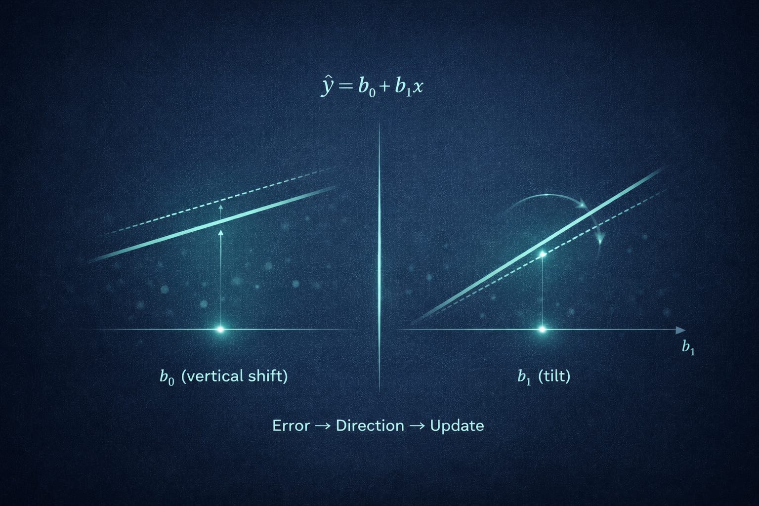
Only after you can see those knobs clearly is it useful to name them. We call the baseline the intercept and the steepness the slope. We call both knobs parameters, because they are values inside the model that we can set.
The rule is written as:
Here (b₀) is the intercept and (b₁) is the slope.
Worked example (making predictions).
Suppose we pick (b₀ = 1) and (b₁ = 2). Then:
If (x = 3), substitute directly:
If (x = 0), the prediction is just the intercept:
Nothing mysterious is happening yet. Training will simply mean: choose (b₀) and (b₁) so that these predictions align well with reality.
Noise: the reason the line will never please everyone
Even if there is a true underlying relationship, your observed points almost never sit perfectly on a line. This is not because your data is “bad”. It’s because the world contains more variation than your measurement captures.
Sometimes the noise is literal measurement error: a sensor has jitter, a scale is miscalibrated, a human labeler is inconsistent, a number gets rounded. Sometimes it’s behavioral variability: two people can receive the same input and respond differently for reasons you didn’t measure. And often it’s missing variables: you’re modeling (y) with one feature (x), but the real system depends on many factors.
A useful mental model is:
there may be a clean trend,
but each observed point is the trend plus “everything else”.
Linear regression doesn’t deny “everything else”. It just refuses to model it explicitly. It says: I will capture the main direction with a line, and I will treat the leftovers as noise.
That makes the phrase “the line doesn’t hit all points” feel normal rather than suspicious. In fact, if your line hits every point exactly, you should be cautious: either the problem is artificially clean, or you’ve accidentally let the model become too flexible (overfitting in disguise), or you’re evaluating on the same data you trained on in a way that hides generalization error.
Noise is also why humility matters in ML. If the data-generating process is noisy, then a perfect predictor might not exist even in principle. The best you can do is reduce uncertainty and make useful probabilistic or average-case predictions. Linear regression is the first model that gently forces you to accept that “some error” is not failure - it’s reality.
The first key idea: error is not embarrassment, it’s feedback
Once you accept that a line cannot satisfy every point, you need a different relationship with “being wrong”. In machine learning, error is not embarrassment. Error is the mechanism by which learning happens.
Take a point ((xᵢ, yᵢ)). Your model predicts (ŷᵢ). The difference between (yᵢ) and (ŷᵢ) is not abstract - it is a visible vertical gap on the scatter plot. If the point lies above the line, the model predicted too low. If it lies below the line, the model predicted too high.
This matters because it turns learning into a loop:
make a prediction using your current parameters,
compare the prediction to the truth,
use the comparison to decide how to adjust.
Without step (2), you have no guidance. You can “guess” different lines, but you cannot say which direction is improvement. So the core requirement for training is not cleverness; it is a consistent way to measure misses.
A subtle point: the error must be defined in a way the model can respond to smoothly. If tiny parameter changes cause unpredictable swings in the error measure, learning becomes chaotic. Linear regression with standard error definitions behaves nicely, which is another reason it’s such a good first model: the feedback is stable enough that you can build intuition about iterative improvement.
So in this section, the main idea is psychological as much as technical: errors are not shameful artifacts to hide. They are the signal that drives parameter adjustment.
💡 What if being wrong is the whole point?
In machine learning, mistakes aren’t something to hide - they’re the mechanism that makes improvement possible.
👉 Subscribe to explore more ideas where math quietly reshapes how we think.
Residuals as a diagnostic, not just a number
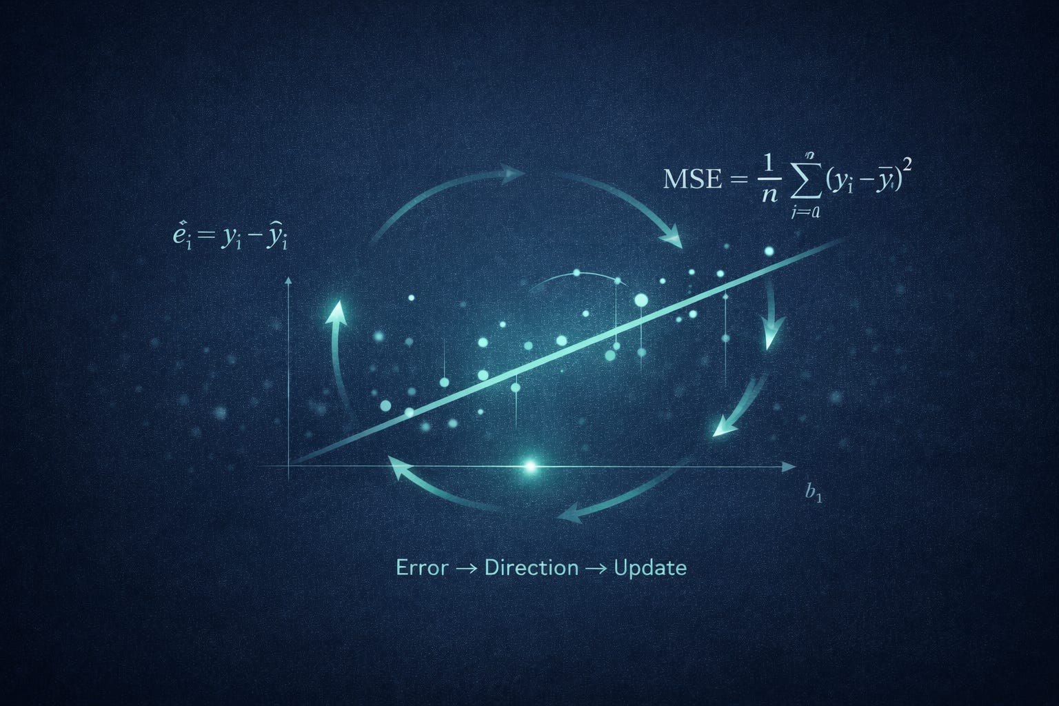
After you’ve stared at those vertical gaps for a while, it’s helpful to name them: they are residuals. For each point (i), we define the residual as observed minus predicted:
And since:
we can write:
The sign matters. If (eᵢ > 0), you underpredicted. If (eᵢ< 0), you overpredicted.
Worked example (computing residuals).
Suppose our data points are:
((1, 2))((2, 3))((3, 5))
and our current line is:
Compute predictions:
at
(x = 1): (ŷ = 1 + 1 = 2)at
(x = 2): (ŷ = 1 + 2 = 3)at
(x = 3): (ŷ = 1 + 3 = 4)
Now residuals (eᵢ = yᵢ - ŷᵢ):
(e₁ = 2 - 2 = 0)(e₂ = 3 - 3 = 0)(e₃ = 5 - 4 = 1)
So far, residuals look “fine”. But the real power is diagnostic: residuals tell stories in aggregate. If residuals are mostly positive for large (x), you’re systematically underpredicting in that region. If they cluster negative for small (x), you’re systematically overpredicting there. Residuals aren’t just numbers - they’re a microscope for model mismatch.
The second key idea: to optimize, you need one score to minimize
Residuals give you many pieces of feedback - one per point. But to choose between two candidate lines, you need a single scoreboard number. Otherwise, you’re stuck arguing about trade-offs point by point: “This line is better here, but worse there”.
This is why loss functions exist. A loss function compresses the whole set of residuals into one number that the computer can minimize.
A common choice is mean squared error (MSE). If you have (n) points, define:
This does two things at once. First, it makes all contributions nonnegative by squaring. Second, it makes “big mistakes” count more than “small mistakes”.
Worked example (aggregating to one score).
Using the residuals from the previous section ([0, 0, 1]), compute MSE:
Square each residual:
(0² = 0)(0² = 0)(1² = 1)
Sum them:
Divide by (n = 3):
Now we can compare lines. A line that produces MSE (0.2) is “better” than one that produces MSE (0.3), under this definition of better. That last clause is important: optimization doesn’t discover goodness; it operationalizes the goodness you defined.
Why squared error feels harsh — and why that harshness is useful
Squared error is opinionated. It says: large errors are disproportionately bad. That can feel harsh, especially if you’re thinking in human terms where a miss is a miss. But squared error is a deliberate choice about priorities.
To see the effect, compare two residual sets:
Set A: ([2, 2, 2])Set B: ([0, 0, 4])
Under absolute error, both have total error (6). Squared error distinguishes them.
Compute squared sums:
For A:
(2² = 4)three timessum (
= 4 + 4 + 4 = 12)
For B:
(0² = 0)(0² = 0)(4² = 16)sum
(= 16)
So squared error prefers A (many small misses) over B (one big miss). That’s the harshness.
Why is that useful? Sometimes it matches reality. In many systems, a few catastrophic predictions cause outsized damage: a medical dose that’s wildly off, a delivery ETA that’s wrong by hours, a credit decision that misprices risk severely. Squared error encodes “avoid disasters even if it means tolerating mild imperfection elsewhere”.
There’s also a computational reason: squaring creates a smooth, bowl-shaped objective for linear regression. Smoothness means that small parameter changes lead to predictable loss changes, which makes optimization stable. If your loss surface has sharp corners, learning algorithms can jitter or stall. So squared error is not only a value judgment; it’s an engineering choice that makes the search landscape easier to navigate.
⚖️ Would you rather tolerate many small misses or prevent one big failure?
Every loss function encodes a value judgment - even when it looks purely mathematical.
💬 Comment - would you design the objective differently?
Optimization as a story of two knobs and repeated correction
Now we return to the two knobs: intercept (b₀) and slope (b₁). Optimization is the process of adjusting these knobs to reduce the loss - usually MSE.
At a human level, you can already anticipate the direction of many corrections. If your line sits too high across the plot - meaning most points fall below it - then most residuals are negative, and lowering the intercept should help. If your line is too low, raising the intercept should help.
Slope is about imbalance across (x). If you underpredict at high (x) and overpredict at low (x), your line is too flat and should tilt upward. If the opposite happens, it’s too steep and should flatten.
The key is that training is rarely a one-shot act. It’s a loop:
pick initial
(b₀, b₁),compute predictions
(ŷᵢ),compute residuals
(eᵢ),compute loss,
adjust
(b₀, b₁)to reduce loss,repeat.
This “tiny edits” framing matters because it generalizes. Even though linear regression can be solved directly with a closed-form formula, most modern ML training feels like this loop. Once you’re comfortable with “we improve by repeated correction”, later ideas - learning rates, convergence, early stopping, optimizer choices - feel like natural refinements rather than arcane rituals.
The goal isn’t to make optimization sound glamorous. It’s closer to careful woodworking: measure, shave a little, measure again. And the more clearly you can connect each shave to the measurement, the more trustworthy the process becomes.
The hill-and-valley picture: turning model fitting into navigation
The optimization loop becomes much easier to reason about once you adopt the hill-and-valley picture.
Imagine every possible pair ((b₀, b₁)) as a location on a map. For each location, you can compute the loss (say, MSE) using your dataset. Now imagine the loss as a height. High loss is a mountain. Low loss is a valley. Training means finding the lowest valley.
This turns a vague task (“fit the model”) into navigation (“walk downhill”). It also clarifies why the loss function is so central. Without a scalar loss, you can’t define height; without height, you can’t define downhill.
For linear regression with squared error, this landscape has a particularly friendly shape: it’s a smooth bowl. Intuitively, if you start from a bad line and move a little in a helpful direction, the loss tends to decrease smoothly; you don’t hit unpredictable cliffs. That’s why the metaphor is not just motivational - it reflects a real mathematical property (convexity) that makes training reliable.
But even if you don’t use that word, the practical takeaway is simple: in this setting, there aren’t many “competing explanations” with similar loss. There is a single best region. So if your training is unstable, it’s often because of the step size, data scaling, or implementation - problems you can fix - rather than because the landscape itself is treacherous.
This mental picture is also a bridge to gradient descent: if you can estimate the local slope of the terrain, you can decide where to step next.
Gradient descent: learning by taking steps you can justify
Gradient descent can be introduced without derivatives by asking a plain question: if I nudge a knob slightly, does the loss go up or down? If nudging (b₁) upward makes the loss smaller, you should increase (b₁). If it makes the loss bigger, you should decrease (b₁). Do the same for (b₀). Repeat.
Derivatives enter as the clean, efficient way to compute those “nudges” without trial-and-error probing. They tell you how sensitive the loss is to each parameter.
Let’s derive the gradients for MSE step by step, carefully.
Start with:
Residual is:
And prediction is:
So:
Differentiate (L) with respect to (b₀). Use the chain rule:
Since (eᵢ = yᵢ - b₀ - b₁ xᵢ),
So:
Similarly for (b₁):
But:
So:
Gradient descent updates:
Here (𝛼) is the learning rate: too large and you overshoot; too small and you crawl.
Worked example (one gradient step).
Data: ((1, 2)), ((2, 3)). Start (b₀ = 0), (b₁ = 0).
Predictions: (ŷ = [0, 0]). Residuals: (e = [2, 3]).
Initial MSE:
Gradients:
Choose (𝛼 = 0.1). Update:
New predictions: at (x = 1), (ŷ = 1.3); at (x = 2), (ŷ = 2.1). Residuals: (0.7, 0.9).
New MSE:
One justified step took loss from (6.5) to (0.65). That’s the learning loop in miniature.
A concrete walkthrough: hours studied vs. exam score
Now let’s step away from arithmetic and return to the lived feel of training.
Imagine a dataset of students: hours studied (x-axis) and exam score (y-axis). You plot it and see the usual mess. Some students studied a lot but scored poorly - sleep deprivation, stress, test anxiety, maybe they focused on the wrong topics. Some studied little but scored well - prior knowledge, strong intuition, lucky question coverage. But despite the chaos, the cloud leans upward: more studying tends to help.
Suppose your initial line is too flat. Conceptually, that means it doesn’t “respect” the upward lean of the data. What happens to residuals? On the right side (high study hours), the points tend to sit above your line. Those are positive residuals: you underpredicted the high-study students. On the left side (low study hours), points tend to sit below your line. Those are negative residuals: you overpredicted the low-study students.
That residual pattern is not random noise; it’s a coherent critique. It’s the dataset saying: “Your slope is too small”.
So the optimizer increases the slope a little. As the slope increases, the right end of the line rises (helping underpredictions on high study hours) and the left end drops relative to before (helping overpredictions on low study hours). The loss decreases.
Then you might notice something else: perhaps the line is now consistently too low overall. That would show up as many positive residuals across the board, suggesting the intercept should increase. Training becomes a repeated, almost conversational adjustment: tilt, shift, re-check. Not until it’s perfect - until further adjustments stop making meaningful improvements.
What “best fit” really means: the line that makes the fairest trade-offs
“Best fit” is a dangerously friendly phrase, because it sounds like the line should match as many points as possible. But in noisy data, matching many points exactly is not the goal - and often not even possible.
Under squared error, the “best” line is the one that minimizes MSE:
That definition implies a particular kind of compromise. Every data point gets a vote, and the line positions itself to make the total squared discomfort as small as possible. It will not satisfy the outliers, and it will not satisfy every region equally. Instead, it makes trade-offs according to the rules encoded in the loss function.
This is why I sometimes describe optimization as producing a notion of “fairness”, but a very specific, mechanical fairness: fairness as defined by the objective. Squared error gives more influence to points with large residuals, because shrinking a large residual yields a big loss reduction. If you used absolute error, you would get a different “fair” compromise. If you weighted certain points more heavily (for example, high-value customers), you’d get yet another.
This framing helps you avoid a common confusion: if the fitted line doesn’t look like what you expected, it may not be “wrong.” It may be doing exactly what you asked under your chosen loss - especially if the dataset contains outliers, nonlinearity, or heteroskedastic noise (changing variance). “Best fit” is not a platonic ideal. It’s the best answer to a question you defined.
The model’s humility: what linear regression refuses to claim
A straight line can’t express a threshold, a curve, a plateau, or an interaction - at least not without additional feature engineering. If the real relationship is “benefit increases quickly at first, then levels off”, a line will insist on one constant rate of change. If the real relationship is “nothing happens until (x) crosses a boundary”, a line will smear that boundary into gradual change. If two variables interact (say, studying helps only if you also sleep enough), a single-feature linear regression can’t see that at all.
This is not a bug. It is the consequence of choosing a simple explanation on purpose.
There’s a kind of integrity in that refusal. Linear regression will not pretend to have discovered a complex mechanism. It will tell you only what fits inside its vocabulary: an overall trend plus a baseline. That’s why it remains a foundational learning tool - because it makes the boundary between “what the model can say” and “what the world might be doing” very clear.
In practice, this humility makes linear regression useful even when it’s not “the best predictor”. It’s often an excellent baseline and a strong diagnostic. If a complex model claims huge gains over linear regression, you can ask: is the relationship truly nonlinear, or did the complex model pick up leakage, spurious correlations, or noise? If linear regression performs surprisingly well, that’s also information: perhaps your problem is dominated by a simple trend, and you should focus on data quality, measurement, and feature design rather than architectural complexity.
Learning to appreciate what a model refuses to claim is a deep ML habit. It keeps you honest, and it keeps your systems more stable.
When optimization can’t save you: the failure modes that look like “bad training”
There are times when you can do everything “right” in training - correct code, stable optimization, convergence - and still feel disappointed. This is not always a training problem. Often it’s a problem of mismatch between the model family, the features, and the world.
If the true relationship is curved, no amount of optimizing a line will remove structure from the residuals. You can minimize MSE perfectly within the space of lines and still see a systematic pattern: residuals positive in the middle and negative at the ends, or vice versa. That pattern is a clue that your explanation vocabulary is too small.
If an important variable is missing, the model will treat its influence as noise. Imagine predicting exam score from hours studied but ignoring sleep. The model will “see” sleep as unexplained variability. Your residuals will be larger than they need to be, and you may falsely conclude the problem is inherently unpredictable.
Outliers are another classic failure mode, especially under squared error. Since squared error punishes large residuals heavily, a few extreme points can tug the line away from the majority. The optimizer is not misbehaving; it is faithfully minimizing the objective you gave it. If those outliers are measurement errors, this is painful. If they are legitimate rare cases, you have a real trade-off: do you want to serve the typical case well, or do you want to reduce catastrophic failures on rare points?
The practical lesson is: when results look like “bad training”, ask whether the model is actually failing to optimize - or whether it is optimizing something reasonable over a representation that cannot capture the structure you care about.
Common misunderstandings: where beginners talk themselves into the wrong conclusion
Linear regression is interpretable, which is wonderful, but it also invites overconfident storytelling.
A big one is causation. A fitted slope does not mean (x) causes (y). It means that within your dataset, variation in (x) is associated with variation in (y), after whatever other features you included (if any). Confounders can create impressive slopes that vanish when you measure the right variables. Correlation is not a technicality - it’s the default state of observational data.
Another misunderstanding is treating the slope as a law of nature. The slope depends on the population you sampled, the range of (x) values present, and the other variables you did or did not include. Add a new feature and the slope can change, not because the world changed, but because you changed what the model is allowed to attribute to each feature.
A third trap is trusting a single summary metric too much. MSE can look “good” while the model makes systematic errors in certain ranges of (x), or for certain subgroups. You need residual plots and slice analysis to see whether the errors are randomly scattered (a sign you’ve captured the main structure) or patterned (a sign you’re missing something).
Closing: the real heartbeat is “define error, then minimize it”
If you zoom out far enough, linear regression stops being “about lines” and becomes “about learning as disciplined correction”.
You start with a parameterized rule - a rule with knobs. You don’t pretend it’s true. You simply commit to a vocabulary of explanations you’re willing to use. Then you define what it means to be wrong in a way that is explicit and computable. That definition becomes a single objective number. And once you have a number, you can improve the rule by changing the knobs to reduce it.
That is the heartbeat: define error, then minimize it.
Everything else - residuals, squared loss, gradients, learning rates - is structure built around that rhythm to make it reliable. Linear regression is the cleanest place to hear the beat without distractions. The moment you internalize it, later models feel less like magic. A neural network is not an alien artifact; it is the same loop with more knobs. A large language model is the same loop at enormous scale. The details matter, of course - but the mindset transfers.
There’s also a quiet reassurance in this. Machine learning can look like a zoo of architectures and acronyms. Linear regression reminds you that, underneath, we’re doing something modest and human: we propose a simple story, we listen to how it fails, and we revise the story according to a rule we can explain. If you can do that with a line, you’re already thinking the way the rest of machine learning asks you to think - even when the models stop looking like lines.
❤️ If you felt the heartbeat…
The mindset behind linear regression is the same one powering neural networks and language models - just scaled up.
🔁 Share this with someone learning machine learning - it might save them years of confusion.
An Introduction to Statistical Learning: with Applications in Python (Springer Texts in Statistics) 2023rd Edition by Gareth James, Daniela Witten, Trevor Hastie , Robert Tibshirani, Jonathan Taylor
The Elements of Statistical Learning: Data Mining, Inference, and Prediction, Second Edition by Trevor Hastie, Robert Tibshirani, Jerome Friedman
All of Statistics: A Concise Course in Statistical Inference (Springer Texts in Statistics) by Larry Wasserman
Pattern Recognition and Machine Learning (Information Science and Statistics)
by Christopher M. Bishop
Stanford CS229 notes (linear regression + optimization) by Andrew Ng and Tengyu Ma