
From lines to layers: How Linear Regression shaped the foundation of modern Machine Learning
Machine Learning and Artificial Intelligence


Imagine you have a sunny backyard where you’ve been growing a bunch of magical bean plants. Every morning, you fill up a watering can with a certain number of cups of water - maybe 1 cup one day, 3 cups another day and gently pour it over your plants. After a few weeks, you notice that some of your plants are much taller than the others, and you start to wonder
“Is giving more water the secret to making them grow taller?”
“How can I predict how tall they’ll be next time I try a different amount of water?”

You’ve got a notebook where you recorded each plant’s daily water and its final height after two weeks. Let’s say you have ten plants, each with a cute name - like Benny, Twinkle, Sprout, and so on.

Benny got 6 cups a day and is now 14 inches tall. Twinkle got 8 cups a day and is 18 inches tall. Sprout got 4 cup a day and is 10 inches tall. At first, these numbers seem random, but you have a hunch: the more cups of water, the taller the plant. Yet you don’t want to just guess anymore - you draw the points to figure out a more precise way.
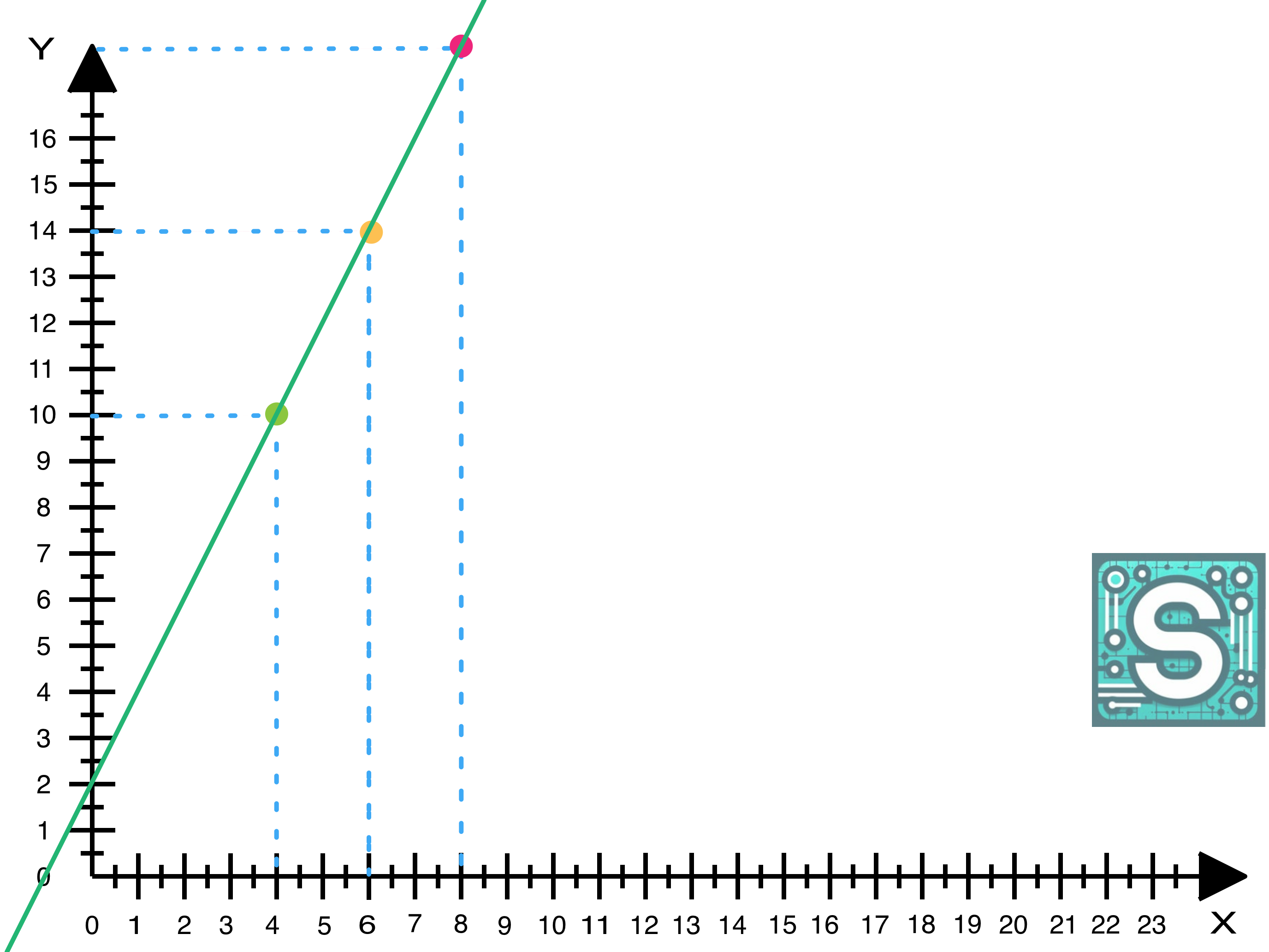
Now you have a bunch of pairs (x, y): cups of water (x) and plant height (y).
Benny: (x=6, y=14)
Twinkle: (x=8, y=18)
Sprout: (x=4, y=10)
Then you draw them as dots on a graph - maybe the x-axis is cups of water and the y-axis is plant height. Plotting these on a graph, you’d see they form a line.
The formed line can be described by a Linear Function. And process of finding that function is called a Linear Regression. It is acting like a special pair of glasses that helps you see the invisible line linking “cups of water” to “plant height”.
Understanding the Linear Function: What it looks like and how it works
When we talk about a Linear Function (especially in the context of Linear Regression), we usually write it like this:
y is the output value, the value we want to predict (like the height of a magical bean plant).
x is the input value, in this case the value we measure (like the cups of water given to the plant).
w0 (the intercept) tells us the starting point of the line - imagine where your line crosses the y-axis when x=0.
w1 (the slope) tells us how steep the line is how much y changes when x increases by 1.
A basic 2D plot helps us see this visually. Let’s pick a baseline linear function.

If you change w0 (the intercept):
When increased (2 → 4), the entire line moves up along the graph.
When decreased (2 → 0), the entire line moves down along the graph.
This is like saying, “What if the plant starts out taller or shorter with no water at all?”.

If you change w1 (the slope):
The line tilts more steeply (0.5 → 1).
The line tilts flattens out (0.5 → 0.25).
A big slope means lots of growth per cup of water; a small slope means just a little bit of growth.
By the way, we could also write our formula as follows:
But let’s stick to more formal, math naming.
Perfect Fit Scenario: What happens if points lie exactly on a line?
Imagine you gather three magical bean plants and measure how much water each got and how tall they grew. In this perfect fit example, let’s say the data points land exactly on a straight line:
Benny: (x=6, y=14)
Twinkle: (x=8, y=18)
Sprout: (x=4, y=10)
Because these points fit perfectly on some line
we can solve for w0 and w1 directly without any leftover errors.
Use two data points to solve for your intercept (w0) and slope (w1). For instance, compare Benny and Twinkle:
for Benny:
\(14=w_0+w_1\times 6 => 14-w_1\times 6=w_0\)for Twinkle:
Now let’s substitute w0 obtained from Benny.
Since we know w1, we can now use it to compute w0.
Check the third point (Sprout) to confirm the line is indeed perfect:
which matches y=10. No error at all!
So, our best-fit line (in this rare, perfect scenario) is:
In the real world, data rarely lines up this neatly most of the time, we deal with noisy points scattered around. However, walking through a perfect scenario helps us understand the core idea: if the points do sit exactly on a line, we can find them with simple algebra. This sets the stage for the more general (and more realistic) cases where we have to minimize errors because the points don’t fit perfectly. Understanding this perfect-case math first makes it easier to grasp how we handle imperfect, real-world data later on!
Real-World Data: Why points typically don’t fit perfectly and what that means
In the real world, data is rarely squeaky clean it often has what we call noise. This means if you plot your measurements, the points might hover near some line or curve but won’t sit exactly on it. Perhaps you water your bean plants by hand one day and accidentally spill a bit more than planned, or the sunlight changes or the soil quality varies any of these can cause your carefully noted data to scatter.

Because true perfection is hard to come by, our data ends up with natural variations or even measurement errors. That’s why you’ll rarely see points forming a tidy, straight line in a real experiment. Understanding that your data won’t align perfectly is crucial it sets the stage for how you approach finding relationships in practice. Rather than solving for a single, exact line (like in our perfect-fit example), you need to think about finding the line that’s closest to all those scattered points, acknowledging that there will always be some imperfections.
Let’s see what happens in the situation when we have imperfect data:
Benny: (x=6, y=13)
Twinkle: (x=8, y=18)
Sprout: (x=4, y=11)
Use two data points to solve for your intercept (w0) and slope (w1). Let’s start with Benny and Twinkle again:
for Benny:
for Twinkle:
Now let’s substitute w0 obtained from Benny.
So the linear equation is:
Check the third point (Sprout) to see the imperfection. Now, we substitute x with 4:
which does NOT match y=11!
Given that noisy data is the norm, our goal shifts from finding an exact solution to finding a “best fit”. In Linear Regression, “best” typically means minimizing some measure of how far off your predictions are from the real observations - often using the sum of squared errors. This idea of minimizing overall error is the backbone of how we handle real-world datasets, ensuring we find a line or model that does the best possible job at capturing the underlying trend, even if it’s never a perfect match.
Least Squares intuition: What errors look like and how we minimize them
In Linear Regression, the error (also called a residual) is the vertical distance between a data point and the line we’ve guessed. Formally, the residual is defined as follows:
where
When you plot your data points on a 2D graph (say, plant heights on the y-axis vs. water cups on the x-axis), some points will be above the line and some below.

The difference (marked as blue) between the point’s height and the line’s height is the error.
Squaring the Errors
We often use the sum of squared errors as our measure of “badness”. Instead of just measuring the distance
we square it to get
Why do this?
Punish Large Errors: Squaring a big number makes it even bigger, so if our line is way off for any point, it really ramps up the total error.
Mathematical Smoothness: Squaring is differentiable, which lets us use calculus (like gradient descent) to find where the total error is minimized.
Visualizing the Squares
Imagine drawing a tiny square whose sides are each “error units” long one side goes up/down from the line to the point, and one side goes sideways the same length.

The area of that square is the square of the error. Summing all these little squares from every point tells us how “bad” our line’s predictions are overall.
Minimizing the Total Error
We add up all those squared distances often written as
into something called the cost function or loss function. Our task is to adjust the line (its slope and intercept) until that sum of squares is as small as possible.
Differentiable Objective
Squaring the errors creates a smooth function of our model parameters. This smoothness is what lets us use powerful tools like gradient descent or direct formulas (the “normal equation”) to find the best set of (w0, w1).
Proven Track Record
The least squares method has been around for hundreds of years (Gauss, Legendre, and other famous mathematicians developed and used it). It remains a cornerstone of statistical analysis precisely because it’s:
Simple to implement
Effective in many scenarios
Mathematically robust
In a nutshell, squaring errors is our way of balancing all the differences between the line and the real data. It’s central to how Linear Regression figures out which line best explains your messy, real-world points.
Mathematical Derivation: How to use derivatives to find w0 and w1
In Linear Regression, we define a cost function - often the Sum of Squared Errors (SSE) - to measure how far our predictions are from the real data. Let’s use SSE in our case:
where:
m is the number of data points,
xi and yi are the feature and target values for the i-th data point,
w0 and w1 are the parameters we want to find.
To minimize this cost function, we use calculus - specifically, partial derivatives. Here’s the procedure.
Write Down the Cost Function
Take Partial Derivatives
We compute two derivatives: one with respect to w0, another with respect to w1:
Set Each Derivative to Zero
To find the minimum of SSE, we solve:
Solve the Resulting Equations
After some algebra, you’ll arrive at the normal equations for w0 and w1. In practice, for a simple linear regression (one feature x):
where:
Calculus provides a systematic, precise method to locate the parameters that make the sum of squared errors as small as possible. Rather than guessing or eyeballing, we have a mathematical guarantee that by setting these derivatives to zero, we’re finding the best possible line for our data at least, in the sense of minimizing total squared error. This approach underpins almost all of classical linear regression and extends to many more advanced machine learning algorithms that rely on gradient-based optimization.
Solving for the Best-Fit Line: What the final equations mean
The above formulas come directly from setting the partial derivatives of the sum of squared errors to zero (as shown in the previous steps). Let’s break down the components:
These tell us where the “center” of our data lies.
This measures how in sync changes in x are with changes in y.
If x tends to be above its average when y is above its average (and below when y is below), the sum is larger.
This represents the spread of the x-values around their mean.
If all x points are nearly the same, the denominator stays small - which affects the slope calculation.
This formula combines both terms above. In essence, w1 is a ratio of how strongly x and y move together vs. how much x varies on its own.
Once w1 is found, the intercept w0 ensures the best-fit line passes through the point
In other words, we “anchor” our line so that on average, it fits our data as well as possible.
Exact, Analytical Solution: You don’t need to guess and check or use iterative methods if you have a small-ish dataset. You can calculate the best parameters directly.
Fast for Small Datasets: For a single feature (and even for multiple features in moderate numbers), this approach is typically very quick to compute.
Foundation in Statistics: These formulas have been around for centuries and are mathematically guaranteed to find the global minimum of the sum of squared errors - no local minima surprises here!
In short, these Normal Equations are a cornerstone of simple linear regression, illustrating both the mathematical elegance and practical speed of finding the best-fit line when the data is not too large.
Example: Benny, Twinkle, Sprout
We are ready to calculate the best-fit line to predict the height of magical bean plants. Let’s imagine you recorded imperfect data in your notebook.
Benny: (x=6, y=13)
Twinkle: (x=8, y=18)
Sprout: (x=4, y=11)
Now, the gole is to obtain w0 and w1.
Derived formula to obtain w0 is
and to obtain w1 is
So the formula for the line is as follows.
When you plot obtained linear function, you can easily notice data points don’t lie exactly on the line, but are really close to it.

If you didn't water your plants at all, they would grow to be 3.5 inches tall. At the same time, you can now predict that if you watered your plants 10 coups a day, they would grow to be 21 inches tall.
From Lines to Layers: What Neural Networks share with linear regression
Imagine a Neural Network as a digital brain that helps computers learn and make decisions, just like how our brains do! It’s made up of layers of “neurons” (tiny processing units) that work together to understand patterns and solve problems.

The Input Layer: Think of the first layer of a neural network like a group of sensors. For example, if you’re showing it pictures of cats, the input layer receives raw information - like the colors and shapes in the image.
Hidden Layers: The real magic happens in the hidden layers. These layers take the input, process it, and figure out patterns. For example, the network might learn to spot things like ears, whiskers, and tails if it’s analyzing cats. Each neuron in the hidden layer takes a small piece of the input, processes it, and passes it along.
Here’s the cool part: these neurons work together to discover complex patterns - not because they’re told how, but because they learn from the data itself.
The Output Layer: Once the hidden layers have done their job, the output layer gives the result. For example, it might say, "This is 95% likely to be a cat!" or "This is a 3-bedroom house worth $500,000."
At first, a Neural Network doesn’t get everything right. It learns by trial and error, comparing its predictions to the correct answers and adjusting itself (this process is called training). Over time, it gets really good at spotting patterns and making predictions.

Neural Networks, at their core, can be viewed as multiple layers of linear functions (like y = w0 + w1 * x) combined with nonlinear activation functions (e.g., ReLU, sigmoid). Each “layer” transforms its input (like x) into a weighted sum (like w0 + w1 * x), then passes that sum through a nonlinear function to allow the network to learn complex patterns that simple lines can’t capture.
If you peel away those activation functions, you’ll see a chain of linear equations - the same fundamental building block used in Linear Regression - just stacked and interlaced with additional computations to handle non-linearity.
The key to training Neural Networks effectively is still gradient-based optimization:
Define a Cost (Loss) Function: In Linear Regression, we use sum of squared errors; in Neural Networks, it might be cross-entropy (for classification) or MSE (for regression).
Compute Gradients: Just like we took partial derivatives with respect to w0 and w1, a neural network computes partial derivatives with respect to hundreds or thousands of parameters.
Update Parameters: Using gradient descent (or variants like Adam, RMSProp), we nudge each weight in a direction that reduces the overall error, iterating until we reach a (hopefully good) minimum.
So, Linear Regression isn’t just a simple method on its own - it’s the stepping stone that lets you confidently dive into more advanced models, knowing the fundamental building blocks are the same.
Conclusion and future directions: Recap what we learned, how to proceed, and why it matters
Throughout this journey, we explored:
Linear Equation Basics: Understanding
\(y = w_0 + w_1 \times x\)and how intercepts (w0) and slopes (w1) define the line.
Least Squares: Squaring the differences (errors) between data points and our predicted line, then finding parameters that minimize this total squared error.
Derivation & Parameter Estimation: Using partial derivatives to systematically solve for w0 and w1.
Next Steps
Hands-On Coding:
Try implementing linear regression from scratch in Python (using NumPy) or explore libraries like scikit-learn for a more plug-and-play approach
Plot residuals and perform basic assumption checks to ensure a good fit.
Advanced Variants:
Logistic Regression (for classification tasks).
Regularization (Ridge, Lasso) to handle overfitting and correlated features.
Neural Networks for tackling nonlinear relationships - keep an eye on how the same gradient-based methods apply here.
Experiment with real data:
Gather your own dataset (e.g., a simple house price dataset, stock prices, or a personal project) and practice iterating from data cleaning to modeling and evaluation.
Significance
Mastering Linear Regression does more than help you draw a line through points - it introduces you to the fundamental concepts that echo throughout machine learning:
The parameter tuning process (finding w0, w1 or more parameters in complex models).
Error minimization (leveraging derivatives or iterative methods to optimize a cost function).
Model evaluation (judging whether your predictions actually make sense).
By understanding these core ideas, you’re well on your way to tackling more sophisticated algorithms and shaping your machine learning or data science skill set for the future.