Decision Trees — how machines learn by asking questions

Machine learning fundamentals

May 27, 2026

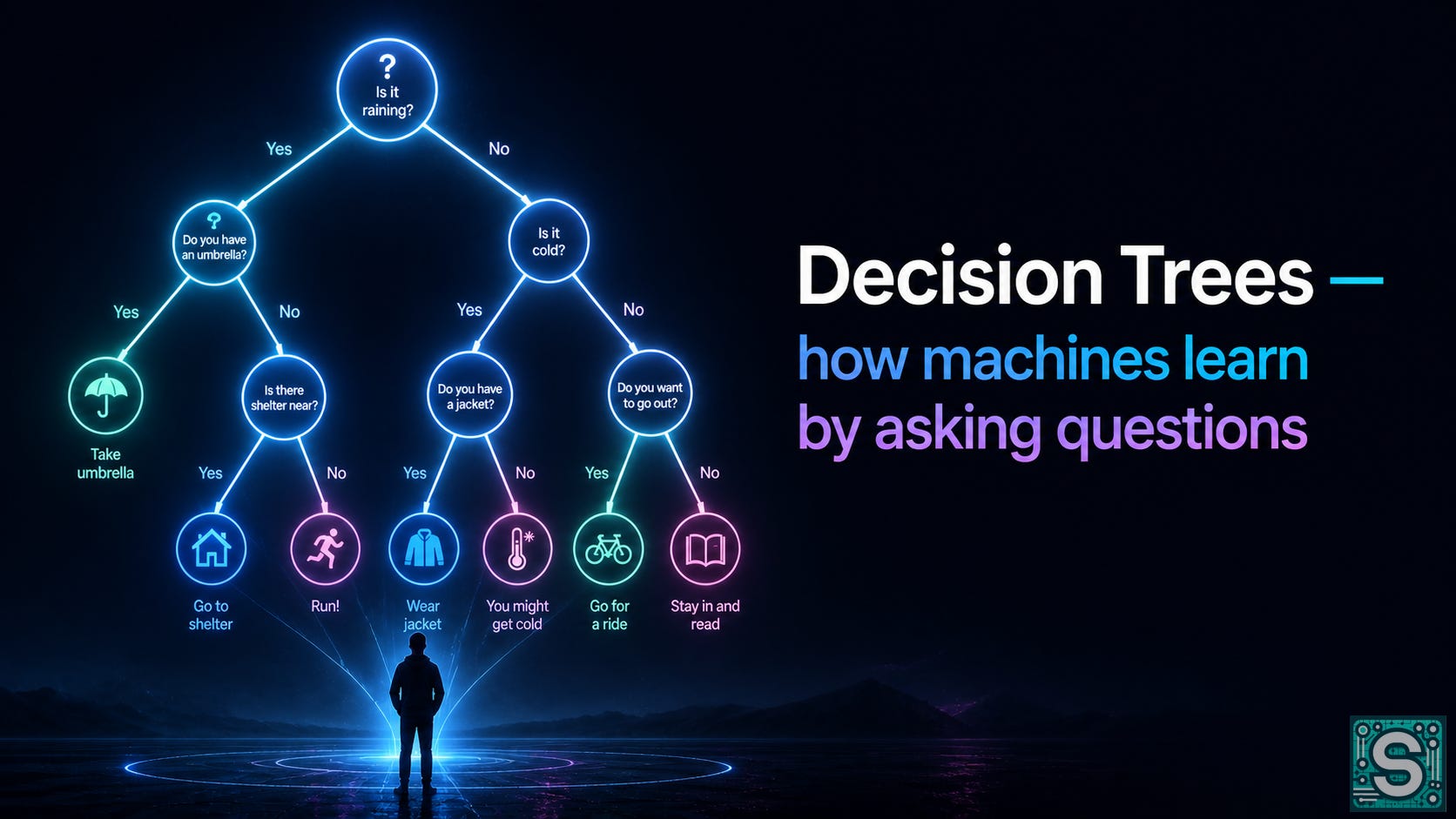
Decision trees are one of the rare machine-learning models that you can explain without asking anyone to suspend disbelief. You can read a tree like you’d read a flowchart. You can often defend its behavior in plain language. And you can usually tell, by inspection, why it fails.

That readability is not an accident. A decision tree is built around a very human idea: if you’re uncertain, ask a question that reduces uncertainty. Then repeat. A tree is a learned sequence of questions - questions the algorithm invents by looking at data - until the remaining ambiguity is small enough that it’s willing to commit to an answer.

In this post I’m going to treat decision trees less like a “model family” and more like a habit of mind: learning as the craft of choosing useful questions. We’ll start with the intuition (why questions help), then get concrete about how a tree proposes and evaluates candidate questions, what “splits” really mean geometrically, why recursion is the natural way to grow a tree, and how stopping and pruning are basically the same human skill: knowing when additional detail stops being insight and starts being noise.

⚡ What if models don’t “think” at all?

Most machine learning systems are just optimizing - adjusting step by step to reduce error. Not intelligence - adjustment.

👉 Subscribe for more intuitive ML explanations.

Along the way, I’ll introduce the simplest mathematical notion behind “good questions”: impurity (how mixed a group is), and information gain (how much a question reduces impurity). I’ll do the arithmetic slowly, with a small worked example, because this is one of those places where the formula only becomes memorable after you’ve computed it by hand once.

If you keep one mental model throughout, let it be this: a decision tree is a conversation with the data. Each internal node asks a question; each branch is the data’s answer; each leaf is the model saying, “Given everything I’ve asked so far, I’m going to predict what most similar past examples looked like.”

A game of “Twenty Questions”, but with a rulebook

Think about the feeling of playing “Twenty Questions” with someone who’s good at it. You start with almost no structure - just a big fog of possibilities. Then come the questions:

“Is it an animal?”
“Is it bigger than a breadbox?”
“Does it have wheels?”

What makes these questions satisfying is not that they’re clever in a literary sense, but that they slice the space of possibilities into chunks that are easier to manage. A great question takes a messy set of candidates and splits it into two groups where each group is, in some way, more coherent than what you started with.

A decision tree is the machine-learning version of that game, except the machine writes the questions for itself. You give it labeled examples - rows of data where you already know the correct answer - and it tries to invent questions that separate the labels as cleanly as possible. Each question is usually yes/no: “Is feature (x) greater than 3.7?” or “Is color equal to red?” So the tree feels like a structured interrogation: one crisp question at a time.

The core promise is simple and surprisingly powerful: if we can turn a messy prediction problem into a sequence of small, clear choices, we can often classify things well. Not because the world is truly made of crisp thresholds, but because thresholds are an efficient way to summarize what you’ve seen. With enough data, and with the right constraints to keep the tree honest, a tree can approximate complicated decision boundaries using only these simple questions.

There’s also a second, quieter promise: interpretability. A tree doesn’t just output “approve” or “deny.” It outputs a path: “income was high, debt was low, history was long… therefore approve”. That path can be wrong, but it is at least legible - which is more than you can say for many other models.

⚡ What if models don’t “think” at all?

Most machine learning systems are just optimizing - adjusting step by step to reduce error. Not intelligence - adjustment. Each step is small, but together they lead to meaningful learning.

🔁 Share it if this made something click.

Why “asking questions” is a useful way to think about learning

At a deep level, supervised learning is about reducing uncertainty. You start with a dataset where labels are mixed together. If you pick a random example from the dataset, you’re not sure what its label will be. Learning is the process of using features to become more sure.

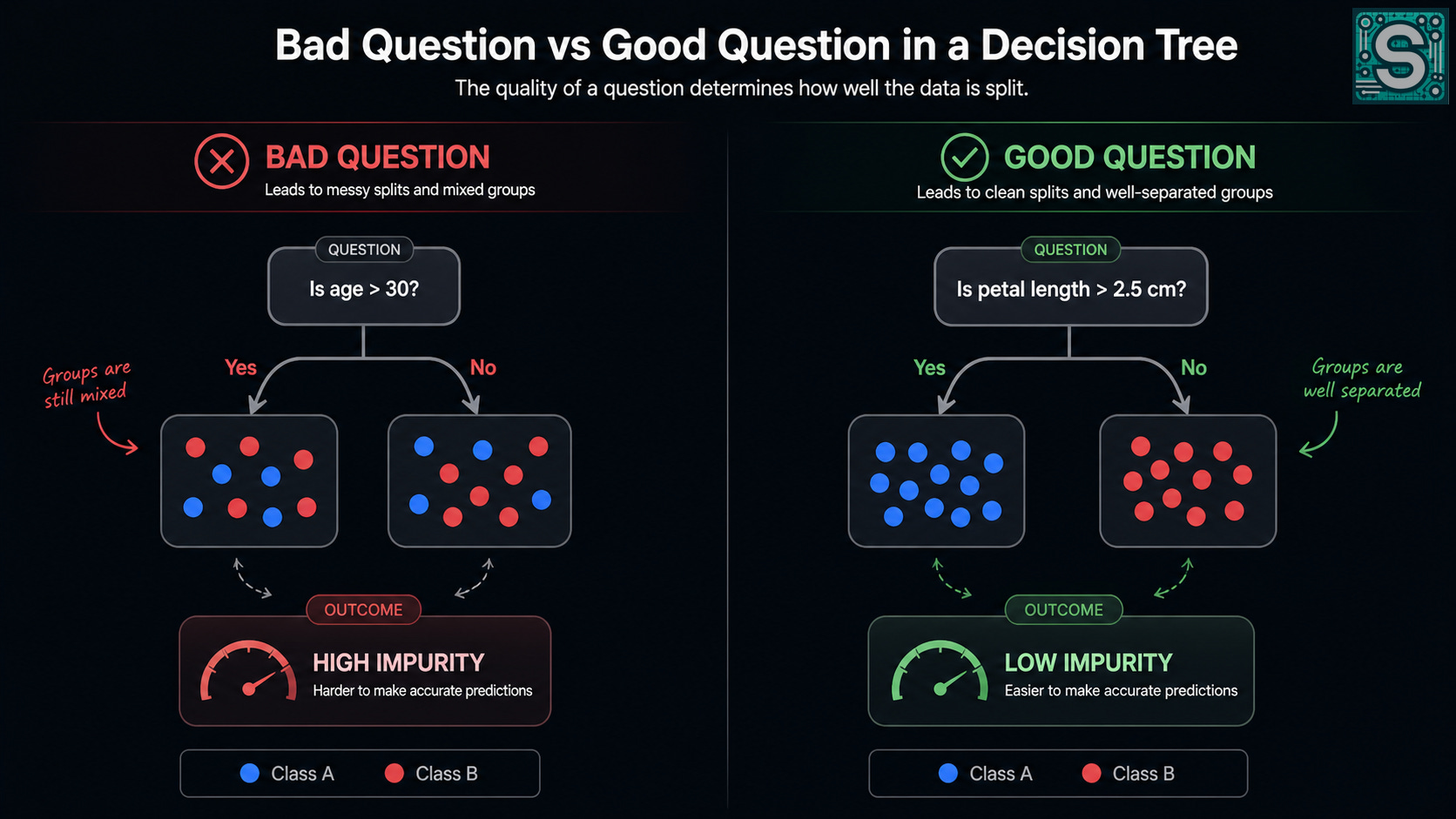
A “question” is useful when it meaningfully reduces that uncertainty. If I ask, “Is the applicant’s favorite color blue?” and the answer has basically no relationship to loan repayment, then the set of possibilities doesn’t shrink in a helpful way. But if I ask, “Is their existing debt above a certain level?” and that tends to separate reliable payers from risky ones, then the two resulting groups become more consistent - more pure.

This idea of purity is the key intuition behind most tree algorithms. A pure group is one where almost everyone has the same label. If a group is pure, you don’t need more questions; the decision is nearly obvious. If a group is mixed, you either need a better question or you accept that your model will have error.

To make that intuition measurable, we use an impurity score. Two common ones are entropy and Gini impurity. I’ll focus on entropy first because it matches the “uncertainty” story very directly.

Suppose a node contains a mix of classes, and let (pᵢ) be the fraction of examples in class (i). Entropy is defined as:

\(H = -\sum_i p_i \log_2 p_i\)

Let’s unpack why this formula matches our intuition, step by step.

We want a score that is 0 when the node is pure. If one class has probability 1, then (p = 1) and (log₂(1) = 0), so the whole sum becomes 0.
We want the score to be largest when classes are evenly mixed. For two classes, that happens at (p = 0.5) and (1 - p = 0.5), which produces a larger value than, say, (p = 0.9) and (0.1).
The (log₂) appears because entropy is measuring uncertainty in “bits”: yes/no questions are naturally base-2. You don’t need to love information theory to use this; you just need to accept that “how surprised should I be?” grows like a logarithm.

Gini impurity is a close cousin:

\(G = 1 - \sum_i p_i^2\)

It has the same qualitative behavior (0 when pure, larger when mixed), and in practice entropy vs. Gini rarely changes your life.

What matters is the mental model: good questions reduce impurity.

From a pile of examples to the first question

A decision tree starts with a pile of labeled examples. Each row is one example; each column is a feature you can measure; and there’s a label you want to predict. For a loan toy example, a row might contain (income, debt, credit-history-length) plus a label like “approved” or “denied” (or perhaps “repaid” vs. “defaulted,” depending on what you’re actually trying to predict).

At the root of the tree, you have every training example mixed together. The algorithm’s first job is to propose candidate questions and pick the one that best sorts the pile into cleaner buckets.

Most tree-building algorithms do something like this:

Choose a feature (say, income).
Choose a threshold (say, income ⩾ 60k).
Split the data into left/right groups based on that question.
Score how much “cleaner” the groups are compared to the parent.

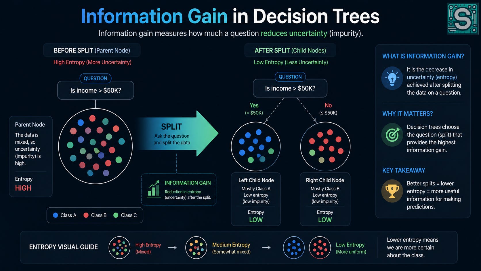
The scoring part is where “information gain” comes in. If you use entropy as your impurity measure, then information gain is literally the reduction in entropy:

\(IG = H_{par} - H_{kids}\)

where (Hkidsᵢ) is the weighted average entropy of the two child nodes:

\(H_{kids} = w_L H_L + w_R H_R\)

and the weights are just proportions of examples:

\(w_L = \frac{n_L}{n}\)

\(w_R = \frac{n_R}{n}\)

That weighted average is important: a split that makes a tiny pure node and leaves a huge messy node is not as impressive as it looks.

Worked example: computing information gain by hand

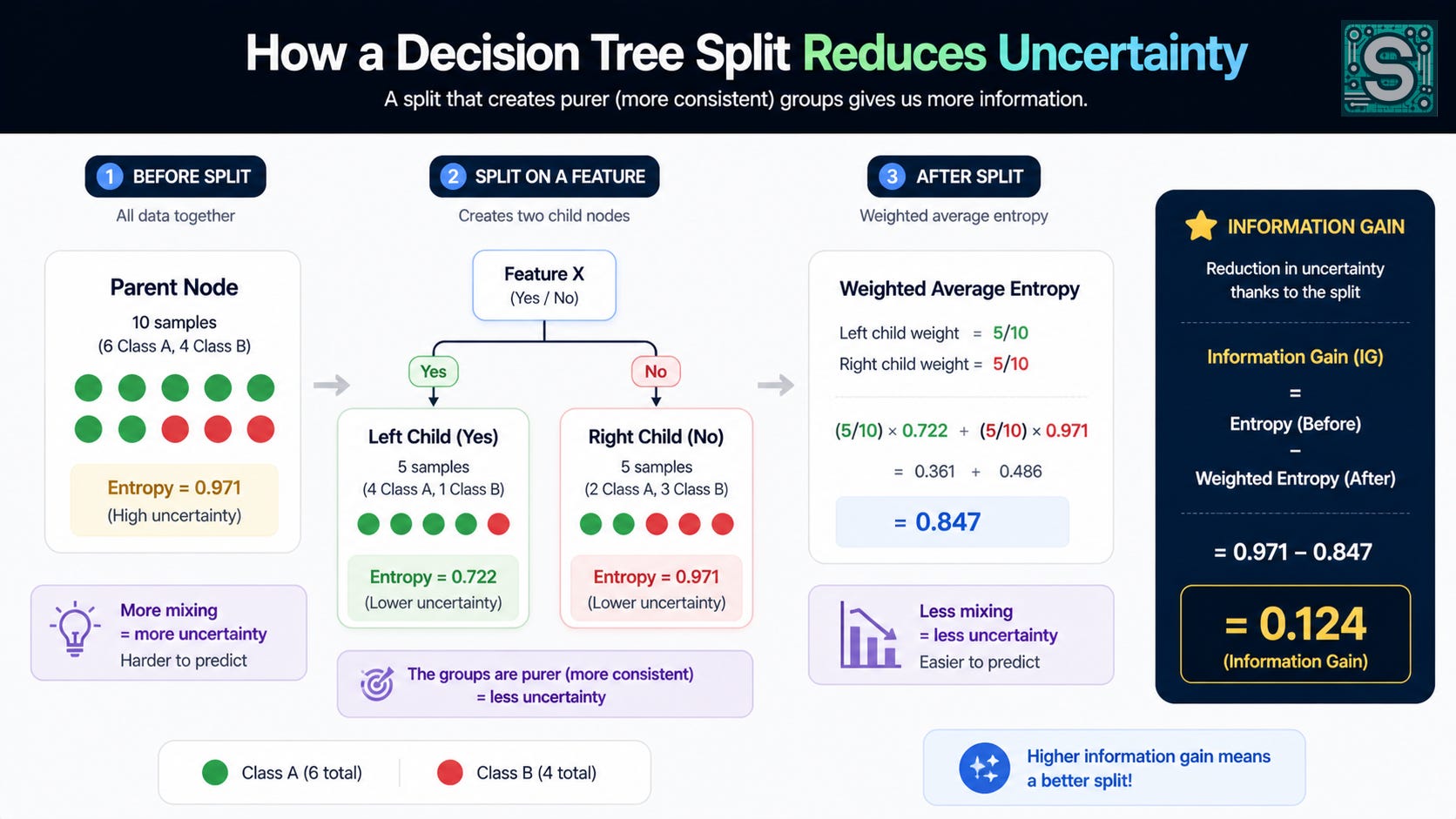
Suppose at the root we have 10 examples:

6 are “approve”
4 are “deny”

So:

\(p_{app} = 6/10 = 0.6\)

\(p_{den} = 4/10 = 0.4\)

Root entropy:

\(H_{par} = -0.6\log_2(0.6) -0.4\log_2(0.4)\)

Now compute the pieces:

(log₂(0.6) ≈ -0.737)
(log₂(0.4) ≈ -1.322)

Substitute:

\(H_{par} ≈ -0.6(-0.737) -0.4(-1.322)\)

\(H_{par} ≈ 0.442 + 0.529 = 0.971\)

Now test a candidate split, like “debt ⩽ 30k”. Suppose it produces:

Left node: 5 examples (4 approve, 1 deny)
Right node: 5 examples (2 approve, 3 deny)

Left entropy:

\(H_L = -0.8\log_2(0.8) -0.2\log_2(0.2)\)

Use:

(log₂(0.8) ≈ -0.322)
(log₂(0.2) ≈ -2.322)

So:

\(H_L \approx -0.8(-0.322) -0.2(-2.322)\)

\(H_L \approx 0.258 + 0.464 = 0.722\)

Right entropy (2/5 approve, 3/5 deny):

\(H_R = -0.4\log_2(0.4) -0.6\log_2(0.6)\)

Notice this is the same numbers as before but swapped, so:

\(H_R \approx 0.971\)

Weighted children entropy:

\(H_{kids} = 0.5(0.722) + 0.5(0.971)\)

\(H_{kids} = 0.361 + 0.486 = 0.847\)

Information gain:

\(IG = 0.971 - 0.847 = 0.124\)

That number, (0.124), is the “value” of this question according to entropy-based information gain. The tree repeats this calculation for many candidate questions and chooses the split with the highest gain.

⚠️ A strong read for founders and leaders ⚠️

Millennial Masters by Daniel Ionescu explores how modern businesses are built and grown — through founder judgment, AI, growth systems, and the leadership behaviors that shape teams long before strategy does.

What a “split” really is: drawing boundaries you can explain out loud

Most of the time, a tree’s questions are not philosophical. They’re just boundaries.

For a numeric feature (x), the question is typically:

“Is (x ≤ t)?”

For a categorical feature (like “has a co-signer: yes/no”), it might be:

“Is category equal to (c)?”

If you’ve ever made a quick human rule like “If the temperature is below 32°F, it might be snow”, you’ve already used the basic shape of a decision-tree split. It’s a threshold rule. The only difference is that the tree learns the threshold (t) from data by checking which threshold produces the cleanest separation of labels.

Geometrically, each split is carving the feature space into regions.

In one dimension (one feature), “(x ≤ t)” cuts the line into two intervals. In two dimensions, you get axis-aligned cuts: “(x₁ ≤ t)” is a vertical line; “(x₂ ≤ t)” is a horizontal line. In higher dimensions, it’s the same idea: hyperplanes aligned with feature axes.

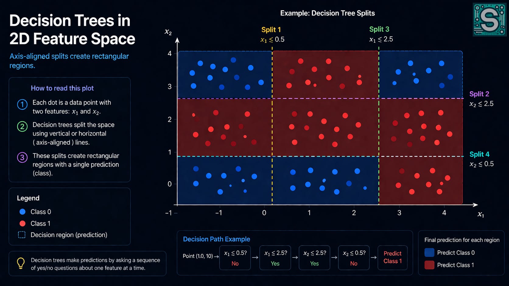
This is where interpretability comes from. A tree’s decision is a conjunction of simple statements:

(x₁ ≤ t₁)
(x₃ > t₃)
category is in {A, B}

You can read them top to bottom and say them out loud. That matters in practice because it makes debugging possible. If a tree is making an embarrassing prediction, you can trace the path and often find the exact question that sent the example down the wrong branch.

There’s a trade-off hiding here, though. Axis-aligned splits are easy to explain, but they can be an awkward fit when the “true” boundary is diagonal or smooth. Trees can approximate those boundaries, but they often need many small steps - many questions-to do it. So interpretability and expressiveness are always negotiating with each other.

Growing the tree one choice at a time

Once you’ve understood the first split, you’ve understood almost the entire tree-growing process, because the algorithm is fundamentally recursive.

Here’s the story the model is telling itself:

At the root, I have a mix of labels.
I will ask one question that best reduces the mix.
Now I have two smaller piles of examples (left and right).
For each pile, I will again ask: “What question best reduces this pile’s mix?”
I keep doing this until I decide I’m done.

The recursion is not just an implementation detail; it’s the essence of how trees “think”. The tree never tries to plan an optimal sequence of questions globally. It doesn’t search over all possible trees (that would be combinatorially enormous).

Instead, it makes a locally greedy choice: pick the best split right now, then repeat inside each branch.

This greediness is both a strength and a weakness. It’s a strength because it makes training fast and conceptually simple. It’s a weakness because a locally best question might block a globally better structure. You can easily construct cases where a suboptimal first split enables much better splits later. But in many real datasets, the greedy heuristic is “good enough”, especially when combined with regularization strategies like stopping rules and pruning.

It also helps to notice what changes as you recurse: the candidate questions are the same types of questions, but they are evaluated on different subsets of the data. A threshold that is useless globally might become useful inside a branch. For example, “income ≤ 50k” might not help much at the root, but once you’ve restricted to applicants with short credit history, income might become decisive.

So a tree gradually carves the world into smaller regions where simpler rules become valid. That is a very general pattern in ML:

complex behavior often emerges from repeating a simple operation many times.

When does the tree stop asking questions?

If you let a tree keep asking questions indefinitely, it will eventually do something that looks impressive and is actually dangerous: it will memorize the training set.

To avoid that, tree-building needs stopping rules - human judgments encoded as hyperparameters. In human terms, you stop asking questions when additional questions stop being “clarifying” and start being “nitpicky”.

Common stopping conditions include:

Purity threshold: If a node is already “mostly one label”, you stop. For instance, if 98% of examples in a node are “approve”, you might accept that as good enough and not try to chase the remaining 2%.
Minimum samples in a node: If a node contains very few examples, any split you learn there is likely to be unstable. It’s like building a theory of human behavior from three anecdotes.
Maximum depth: You cap how many questions can be asked from root to leaf. Depth is a rough proxy for complexity.
Minimum impurity decrease: You only split if the impurity reduction (information gain, Gini decrease, etc.) is “large enough” to justify the added complexity.

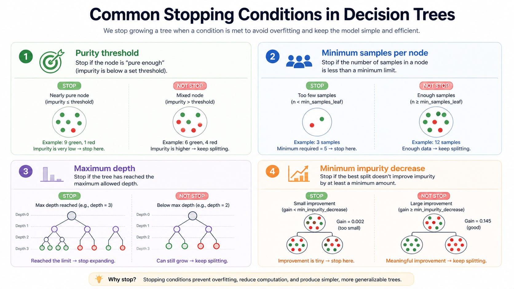
These are all different ways of expressing the same bias: prefer simpler explanations unless the data strongly argues for additional detail.

It’s worth pausing on why stopping is needed even if your training accuracy keeps improving. Training accuracy is a seductive metric because it always rewards complexity. But our real goal is performance on new data. A question that perfectly separates three training points might be capturing an accident: a quirk of measurement, a temporary market condition, or a label error.

So stopping is not a hack. It’s the core generalization idea: we want the model to capture patterns that persist beyond the dataset, and that means refusing to “learn” patterns that are too specific to the sample we happened to collect.

A concrete example: approving a loan by asking a small set of questions

Let’s build a small, intentionally simplified loan-approval story. The goal here is not to propose a real credit policy; it’s to make the mechanics of a decision tree feel vivid.

Assume we train on past applicants with three features:

Annual income (in thousands): (I)
Existing debt (in thousands): (D)
Credit history length (years): (Y)

Label:

\(L \in {\text{Approve}, \text{Deny}}\)

A plausible first question might be about debt burden, because it often separates low-risk from high-risk applicants:

Q1: “Is (D ≤ 25)?”
- If yes, go left (lower debt).
- If no, go right (higher debt).

Inside the low-debt branch, the tree might find that income becomes a clean separator:

Q2 (left branch): “Is (I ⩾ 55)?”
- If yes, most examples might be approved.
- If no, you might need one more refinement.

Now consider those low-debt but lower-income applicants. Perhaps credit history length distinguishes “new to credit” from “stable track record”:

Q3 (left-left branch): “Is (Y ⩾ 3)?”
- If yes, approve (stable).
- If no, deny (too little history).

On the high-debt side, the tree might quickly decide that most examples are denied, but it could still carve out an exception for very high income:

Q2 (right branch): “Is (I ⩾ 90)?”
- If yes, maybe approve (they can service debt).
- If no, deny.

Notice what’s happening: each question is locally reasonable, and the final decision path is something a human could narrate. But also notice the brittleness: “25k debt” and “55k income” are crisp thresholds. In reality, risk changes smoothly, and different datasets would likely push those thresholds around. Still, for many operational settings, a readable rule set like this is extremely useful - even if it’s only an approximation.

Leaves, predictions, and what the tree “believes” at the end of a path

A decision tree’s terminal nodes are called leaves. A leaf is where the tree stops asking questions and produces a prediction.

A key point that beginners sometimes miss is that a leaf is not “a logical conclusion” in some deductive sense. It is a summary of training examples that landed there. If a leaf contains 120 training examples and 90 of them are “Approve”, the leaf’s prediction is usually “Approve”, and it may also store the estimated probability:

\(\hat p(\text{Approve}) = 90/120 = 0.75\)

That estimate is not a deep belief about the world. It’s a frequency statement: among similar examples in the training data, 75% were approved.

Worked example: leaf probabilities and decisions

Suppose a particular leaf contains 8 training applicants:

6 were approved
2 were denied

Then:

\(\hat p(\text{Approve}) = 6/8 = 0.75\)

\(\hat p(\text{Deny}) = 2/8 = 0.25\)

If your tree is doing hard classification, it picks the majority class:

Predict “Approve”.

If you need a score (for ranking or thresholding), you can use (0.75) as a probability-like output. But you should also feel the fragility: with only 8 examples, one mislabeled case changes the estimate from (6/8) to (5/8), i.e., from (0.75) to (0.625). This is why minimum-samples stopping rules matter, and why ensembles (like random forests) are often used to stabilize these estimates.

Also notice something philosophically important: the tree is not “thinking ahead”. It doesn’t say, “If I ask this now, I’ll be able to ask a better question later.” It makes a chain of local choices, and at the end it votes based on what happened to similar past examples.

The quiet trade-off: clarity versus fragility

The reason trees feel so clear is that they commit to a small number of crisp questions. The reason trees can feel so fragile is… they commit to a small number of crisp questions.

A lot of the model’s fate is decided near the root. If the first split changes, then all the downstream splits are learned on different subsets, which means the entire structure can change. Two trees trained on nearly identical datasets can look meaningfully different, not because the algorithm is “random”, but because the choice it makes is often a close call.

Here’s the intuitive mechanism. Imagine two candidate root questions, A and B, with very similar information gain:

Question A produces slightly cleaner groups than B on your current dataset.
You pick A (because that’s what the algorithm does).
Now, inside the left branch of A, you learn a set of follow-up splits specialized to that subset.
If you had picked B, you would have created different subsets, and therefore learned different follow-up splits.

So small data perturbations can cascade. This is particularly visible when:

the dataset is small,
features are correlated (many questions are “almost” equivalent),
labels are noisy,
the optimal split is not sharply better than alternatives.

This is not a reason to dislike trees; it’s a reason to understand what you’re buying. Trees buy you interpretability and the ability to model non-linear, interaction-heavy relationships. In exchange, you accept variance: the learned structure can be sensitive to the sample.

It’s also why tree ensembles are so common. A random forest, in one sentence, is “a way of averaging many fragile trees into a stable predictor”. But even if you later move to ensembles, it’s worth learning single trees first, because they teach you the anatomy of the question-asking process.

Overfitting looks like an over-curious interviewer

Overfitting in decision trees has a particularly relatable flavor. It looks like an interviewer who keeps asking questions - not to understand stable traits, but to memorize one-off details.

A shallow tree might ask:

“Is your income above 60k?”
“Is your debt below 25k?”

A wildly overfit tree starts asking things that are technically true in the training set but not meaningfully predictive:

“Is your income above 61k and your history length exactly 2 years?”
“Did you have a blue mug on Tuesday?” (the human parody of a spurious feature)

What’s happening is that deep trees have enough degrees of freedom to carve the feature space into tiny regions. If you keep splitting, you can often create leaves that contain one or two training examples, at which point the leaf can “predict” perfectly - because it is basically memorizing.

In impurity terms, every split can reduce impurity on training data. If you split until each leaf is pure (all one label), training entropy becomes zero at every leaf. But that is not a victory. That is the model declaring: “I have a special rule for each training case”, which usually generalizes poorly.

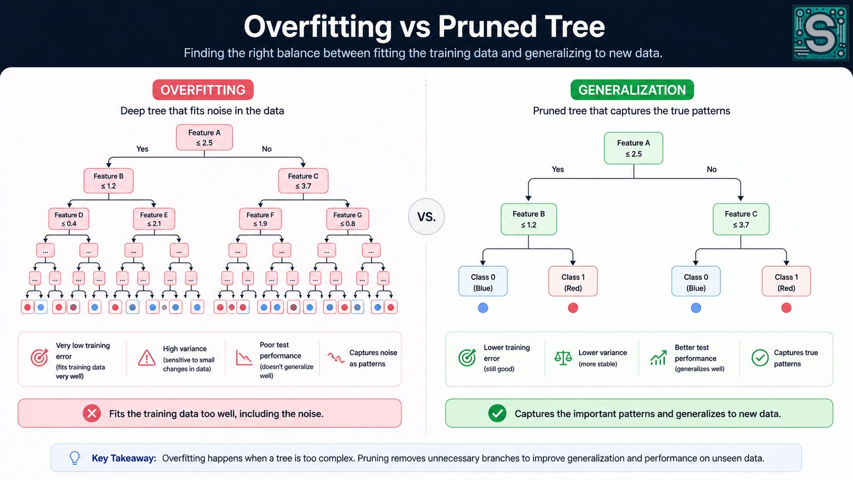
This connects to a broader ML theme: fitting is easy; generalization is hard. Trees make this painfully concrete because the failure mode is visible. You can literally point to a branch and say, “This rule exists only to handle three examples”.

Deep trees can be appropriate when you truly have complex interactions and lots of data. The problem is that depth is a blunt instrument: it increases both expressive power and the ability to chase noise. So you need explicit controls (stopping and pruning) to keep curiosity from turning into memorization.

What pruning is: teaching the tree to shut up at the right time

Pruning is the idea that the tree should be allowed to grow (so it can discover useful structure), but then be encouraged to simplify itself by removing branches that don’t justify their complexity.

There are two broad styles:

Pre-pruning (early stopping): you stop splits during growth using rules like max depth or min samples.
Post-pruning: you grow a large tree, then cut it back.

The intuition behind post-pruning is very human: when you first draft an explanation, you may include lots of details; when you edit, you remove the details that don’t improve the explanation for a new reader. Pruning is editing.

One common formalization is cost-complexity pruning. You balance training error against tree size:

\(J(T) = R(T) + \alpha |T|\)

Let’s interpret each term carefully.

(T) is the tree.
(R(T)) is a measure of how wrong the tree is (often misclassification error on training data, or another impurity-based proxy).
(|T|) is a measure of complexity (often the number of leaves).
(𝛼) controls how much you penalize complexity.

If (𝛼 = 0), you don’t care about complexity and you keep the big tree. If (𝛼) is large, you strongly prefer a smaller tree even if it makes more mistakes on training data.

The core message is not the specific objective. It’s the stance: a simpler tree that generalizes is better than a complicated tree that over-explains the past. Pruning operationalizes that stance by removing branches that look like “exceptions” rather than “patterns”.

Common misunderstandings that trip people up

The first misunderstanding is the most common and the most costly: believing that a decision tree has discovered the true causal rules of the world. A tree discovers a set of splits that are useful for prediction on the data you gave it, under the splitting criterion you chose. That can align with causal structure, but it does not have to.

If, historically, a certain neighborhood correlates with loan default due to economic factors, a tree might split on ZIP code. That could improve prediction, but it is not a causal explanation of repayment behavior, and it might be ethically unacceptable or legally constrained depending on context. Trees are very good at exploiting correlations; they are not automatically good at identifying causes.

A second misunderstanding is about feature “importance”. People often look at the root split and say, “Ah, this must be the most important feature.” Sometimes it is, but not always in a human sense. The root feature is the one that produced the largest impurity reduction at that moment, given:

the available features,
the label distribution,
the greedy nature of the algorithm,
and the specific criterion (entropy, Gini, etc.).

If two features are correlated, the tree might pick one arbitrarily and never use the other, even if both are genuinely predictive. So “appears early in the tree” is not the same thing as “most important in the world”.

A third misunderstanding is believing that trees are always interpretable in practice. A tiny tree with depth 3 is interpretable. A tree with depth 25 and hundreds of nodes is technically readable but practically incomprehensible - like a legal contract that is “just words”. Interpretability is not a binary property; it degrades with size.

So the right takeaway is nuanced: trees can be interpretable, and they often are in constrained form, but you must actively manage complexity if interpretability is one of your goals.

When decision trees shine — and when they struggle

Decision trees shine in settings where the world plausibly behaves like a set of interacting rules, or where we want a model that can represent interactions without feature engineering.

They often feel natural when:

you have a mix of numeric and categorical features,
relationships are strongly non-linear,
feature interactions matter (e.g., “income matters given debt level”),
you care about explanation paths for debugging, policy, or communication.

Trees also handle monotonic transformations and scaling reasonably well, because a threshold split doesn’t care whether income is measured in dollars or thousands, as long as the order is preserved.

Where trees struggle is equally instructive:

Noisy labels: a tree can keep splitting to “explain” noise, unless you stop it.
Small datasets: the best split can be unstable, leading to high variance.
Smooth relationships: if the true relationship is gradual (risk increases smoothly with debt-to-income ratio), hard thresholds can be a crude approximation unless the tree becomes deep.
Extrapolation: trees are poor at extrapolating beyond the range of observed feature values. They partition what they’ve seen; they don’t naturally extend linear trends.

A good rule of thumb is: trees are excellent at carving and categorizing within the observed space, but they can be brittle when the signal is subtle and continuous.

What decision trees teach us about machine learning as a whole

Decision trees are a lesson in how far you can go with a simple learning primitive: choose a question that reduces uncertainty, then repeat. That’s not just a tree idea; it’s a recurring pattern across ML. Many models can be understood as building internal representations that make the label more predictable - trees just do it with explicit questions you can inspect.

They also teach a second lesson that is easy to ignore when you first learn the math: learning from finite data is inherently uncertain. A tree can look like pure logic - clean thresholds, crisp branches, decisive conclusions - yet it is still a statistical object, shaped by sampling variation, label noise, and whatever features you decided to measure. The “logic” is learned, not revealed.

If you take that seriously, you stop expecting a tree (or any model) to hand you the true rules of reality. Instead, you start treating models as tools that compress experience into actionable guidance, with errors that have to be managed, not wished away.

And finally, trees offer a gentle but important moral: interpretability is not the opposite of complexity. A decision tree can be perfectly interpretable at the level of each step, and still be fragile in the overall story it tells. The art is knowing when the next question is real insight - and when it’s the model becoming an over-curious interviewer.

A decision tree is, in the end, a learned conversation with the data. Good tree-building is learning when to keep asking - and when to stop.

🧠 What if complex models are just simple ideas… repeated at scale?

The same mindset behind decision trees powers neural networks - just bigger, deeper, and layered. What looks like complexity is often just repetition.

💬 Did this change how you see machine learning?

slys.dev

Discussion about this post

Ready for more?